Contents
Bayesian Methods for Product Decisions: When and Why to Go Bayesian
A comprehensive guide to Bayesian statistics for product analysts. Learn when Bayesian beats frequentist, how posterior probabilities work, and how to make better decisions.
Quick Hits
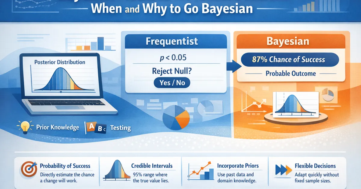
- •Bayesian methods give you the probability a variant wins -- not just whether to reject a null hypothesis
- •Posterior distributions let you quantify exactly how confident you are in every possible outcome
- •Credible intervals mean what most people think confidence intervals mean: a 95% chance the parameter is in this range
- •Bayesian approaches naturally incorporate prior knowledge from past launches, domain expertise, or historical data
- •You can make decisions before a fixed sample size is reached without inflating error rates
TL;DR
Bayesian statistics lets you answer the questions product teams actually care about: "What is the probability this variant is better?" and "How much better is it likely to be?" Instead of binary significance tests, you get full probability distributions over outcomes. This guide covers when Bayesian methods outperform frequentist ones, how posterior probabilities work, and how to integrate Bayesian thinking into product decisions.
Why Bayesian Methods Matter for Product Decisions
The Question Stakeholders Actually Ask
When your PM asks "Did the experiment work?", they want to know: What is the probability that Variant B is better than Variant A?
Frequentist testing answers a different question: "If there were truly no difference, how likely would we see data this extreme?" That is the p-value, and it is not what anyone outside of statistics actually wants.
Bayesian methods answer the real question directly. After running a Bayesian A/B test, you can say:
- "There is a 92% probability that Variant B increases conversion rate."
- "The most likely improvement is 3.2%, with a 95% credible interval of [1.1%, 5.8%]."
- "There is a 78% chance the revenue lift exceeds your minimum threshold of 2%."
These statements are intuitive, actionable, and directly map to business decisions.
When Bayesian Beats Frequentist
Bayesian methods have clear advantages in several common product analytics scenarios:
| Scenario | Why Bayesian Helps |
|---|---|
| Small sample sizes | Priors stabilize estimates when data is limited |
| Early peeking at results | No penalty for checking results before a fixed horizon |
| Decision thresholds | Directly compute P(improvement > minimum threshold) |
| Multiple variants | Posterior comparisons handle many variants naturally |
| Sequential decisions | Update beliefs as data arrives, decide when confident enough |
| Combining data sources | Priors incorporate historical experiments, domain knowledge |
Bayesian methods are not always better. For large-sample, standard A/B tests with a clear primary metric, frequentist methods are simpler and give nearly identical conclusions. The advantage grows when your situation is more nuanced.
Core Concepts for Product Analysts
Posterior Distributions: Your Full Answer
The posterior distribution is the core output of any Bayesian analysis. It tells you the probability of every possible parameter value, given your data and prior beliefs.
In plain language:
- Prior : What you believed before seeing data. Could be "I have no idea" (uninformative) or "Past experiments show lifts are usually 1-5%" (informative).
- Likelihood : How probable the observed data is for each possible parameter value.
- Posterior : Your updated belief after seeing the data. This is what you use for decisions.
For a conversion rate experiment, the posterior might tell you:
import numpy as np

# Simulated posterior samples for conversion rate difference
# (In practice, use PyMC, Stan, or brms to generate these)
np.random.seed(42)
posterior_diff = np.random.normal(0.032, 0.012, 10000)

# Direct probability statements
prob_positive = np.mean(posterior_diff > 0)
prob_above_threshold = np.mean(posterior_diff > 0.02)
median_effect = np.median(posterior_diff)

print(f"P(Variant B is better): {prob_positive:.1%}")
print(f"P(Lift > 2%): {prob_above_threshold:.1%}")
print(f"Median effect size: {median_effect:.1%}")
print(f"95% credible interval: [{np.percentile(posterior_diff, 2.5):.1%}, {np.percentile(posterior_diff, 97.5):.1%}]")
Credible Intervals vs. Confidence Intervals
A 95% credible interval means: "There is a 95% probability the true parameter is in this range." That is what most people assume a confidence interval means, but it is not.
A 95% confidence interval means: "If we repeated this experiment many times, 95% of the intervals would contain the true value." For any single experiment, the true value is either in the interval or it is not.
For product decisions, credible intervals are more useful because they directly quantify uncertainty about the parameter you care about. See Credible Intervals vs. Confidence Intervals for a deeper comparison.
Prior Selection: Encoding What You Know
Choosing a prior is the most discussed aspect of Bayesian analysis. In product analytics, the choice is often straightforward:
- Uninformative / flat priors: Use when you have no prior knowledge. The posterior is driven entirely by data. Results closely match frequentist estimates.
- Weakly informative priors: Use when you know the rough scale. For example, "conversion rate lifts are usually between -10% and +10%." This prevents wild estimates from small samples.
- Informative priors: Use when you have strong historical data. For example, "Our last 20 experiments had a mean lift of 2% with SD of 3%." This borrows strength from past experiments.
See Prior Selection: Informative, Weakly Informative, and Uninformative for detailed guidance.
Bayesian Methods in Practice
Bayesian A/B Testing
The most common entry point. Instead of a fixed-sample test with a binary outcome, you get a posterior distribution over the difference between variants.
from scipy import stats

# Beta-Binomial model for conversion rates
# Control: 1200 conversions out of 10000
# Treatment: 1280 conversions out of 10000

alpha_prior, beta_prior = 1, 1  # Uninformative prior

# Posterior distributions (Beta-Binomial conjugate)
control_posterior = stats.beta(1 + 1200, 1 + 10000 - 1200)
treatment_posterior = stats.beta(1 + 1280, 1 + 10000 - 1280)

# Monte Carlo comparison
n_samples = 100000
control_samples = control_posterior.rvs(n_samples)
treatment_samples = treatment_posterior.rvs(n_samples)

diff_samples = treatment_samples - control_samples

print(f"P(Treatment > Control): {np.mean(diff_samples > 0):.1%}")
print(f"Expected lift: {np.mean(diff_samples):.4f}")
print(f"95% credible interval for lift: [{np.percentile(diff_samples, 2.5):.4f}, {np.percentile(diff_samples, 97.5):.4f}]")
For a complete treatment of Bayesian experimentation, see Bayesian A/B Testing: Posterior Probabilities for Ship Decisions.
Bayesian Regression
When you need to model outcomes with covariates, Bayesian regression provides posterior distributions for every coefficient. This is especially valuable when:
- You have more predictors than observations (priors provide regularization)
- You want uncertainty on predictions, not just point estimates
- You need to combine data across segments (hierarchical models)
See Bayesian Regression: When Shrinkage Improves Predictions and Bayesian Hierarchical Models: Borrowing Strength Across Segments.
Decision Rules with Loss Functions
Bayesian methods naturally integrate with decision theory. Instead of "is p < 0.05?", you minimize expected loss:
def expected_loss(posterior_samples, threshold=0, cost_of_wrong_ship=1, cost_of_wrong_hold=1):
    """
    Compute expected loss for ship vs. hold decisions.
    """
    # Loss from shipping when effect is negative
    ship_loss = cost_of_wrong_ship * np.mean(np.maximum(-posterior_samples, 0))

    # Loss from holding when effect is positive
    hold_loss = cost_of_wrong_hold * np.mean(np.maximum(posterior_samples - threshold, 0))

    return {
        'ship_expected_loss': ship_loss,
        'hold_expected_loss': hold_loss,
        'decision': 'Ship' if ship_loss < hold_loss else 'Hold',
        'confidence': 1 - min(ship_loss, hold_loss) / max(ship_loss, hold_loss)
    }

result = expected_loss(diff_samples, threshold=0.005)
print(f"Decision: {result['decision']}")
print(f"Expected loss from shipping: {result['ship_expected_loss']:.6f}")
print(f"Expected loss from holding: {result['hold_expected_loss']:.6f}")
Comparing Bayesian and Frequentist Approaches
| Aspect | Frequentist | Bayesian |
|---|---|---|
| Output | p-value, confidence interval | Posterior distribution, credible interval |
| Interpretation | "Reject or fail to reject" | "92% probability variant is better" |
| Prior knowledge | Not used | Formally incorporated |
| Multiple comparisons | Requires correction | Naturally handled via joint posterior |
| Sample size | Fixed in advance | Can decide adaptively |
| Computation | Fast (closed-form) | Slower (MCMC sampling) |
| Communication | Difficult to explain correctly | Intuitive probability statements |
For a thorough side-by-side comparison, see Bayesian vs. Frequentist: A Practical Comparison for Analysts.
Getting Started: A Practical Roadmap
Step 1: Start with Bayesian A/B Testing
Replace one frequentist A/B test with a Bayesian version. Use a Beta-Binomial model for conversion rates or a Normal model for continuous metrics. Compare the results -- they will usually agree, but the Bayesian output is easier to communicate.
Step 2: Add Weakly Informative Priors
Once comfortable, incorporate prior information from past experiments. This improves estimates for small-sample tests and prevents unrealistic effect sizes.
Step 3: Move to Bayesian Regression
When you need covariate adjustment or prediction intervals, use Bayesian regression. Tools like PyMC, Stan, and brms make this straightforward.
Step 4: Explore Hierarchical Models
For multi-segment analysis (e.g., experiment effects by country or user tier), hierarchical Bayesian models let you borrow strength across segments while respecting differences.
Common Pitfalls
1. Over-Reliance on Default Priors
Default uninformative priors are fine for standard problems but can produce poor estimates in edge cases. Always check whether your prior makes scientific sense.
2. Ignoring Prior Sensitivity
Run your analysis with multiple priors. If conclusions change dramatically, your data is not strong enough to overcome prior assumptions, and you should collect more data.
3. Treating Posterior Probabilities as Guarantees
A 95% posterior probability is not certainty. Calibrate your expectations -- if you ship every variant with P(better) > 90%, about 10% should still be neutral or negative.
4. Unnecessary Complexity
Not every analysis needs Bayesian methods. For a large-sample A/B test with a clear primary metric, a simple two-sample t-test or z-test is perfectly adequate.
Tools and Implementation
Modern Bayesian computation is accessible through several mature libraries:
- PyMC (Python): General-purpose probabilistic programming. Best for custom models.
- Stan (R/Python/other interfaces): High-performance MCMC. Gold standard for complex hierarchical models.
- brms (R): Formula-based interface to Stan. Easiest on-ramp for R users familiar with lm/glm.
See Practical Bayes: Using PyMC, Stan, and brms for Real Analysis for implementation details.
Related Methods
- Bayesian A/B Testing - Posterior probabilities for ship decisions
- Bayesian vs. Frequentist - Side-by-side comparison
- Credible Intervals vs. Confidence Intervals - What changes with Bayesian intervals
- Prior Selection - Choosing appropriate priors
- Bayesian Sample Size - Planning Bayesian experiments
- Bayesian Regression - Regularized regression with posteriors
- Hierarchical Models - Borrowing strength across segments
- Practical Bayes Tools - PyMC, Stan, and brms
Key Takeaway
Bayesian methods let you directly answer the question stakeholders actually ask: "What is the probability this change works?" Instead of binary reject-or-fail-to-reject decisions, you get full posterior distributions showing how likely each outcome is. This makes Bayesian statistics a natural fit for product decisions where you need to weigh trade-offs, incorporate prior knowledge, and communicate uncertainty clearly. Start with Bayesian A/B testing or Bayesian regression, and expand from there.
References
- https://doi.org/10.1214/06-BA101
- https://mc-stan.org/users/documentation/
- https://www.pymc.io/welcome.html
Frequently Asked Questions
Do I need to know advanced math to use Bayesian methods?
When should I stick with frequentist methods instead?
How do I convince stakeholders to trust Bayesian results?
Key Takeaway
Bayesian methods let you directly answer the question stakeholders actually ask: 'What is the probability this change works?' Instead of binary reject-or-fail-to-reject decisions, you get full posterior distributions showing how likely each outcome is. This makes Bayesian statistics a natural fit for product decisions where you need to weigh trade-offs, incorporate prior knowledge, and communicate uncertainty clearly. Start with Bayesian A/B testing or Bayesian regression, and expand from there.