Contents
Credible Intervals vs. Confidence Intervals: What Changes
Understand the real difference between credible and confidence intervals. Learn what each actually means, when it matters, and how to interpret both correctly.
Quick Hits
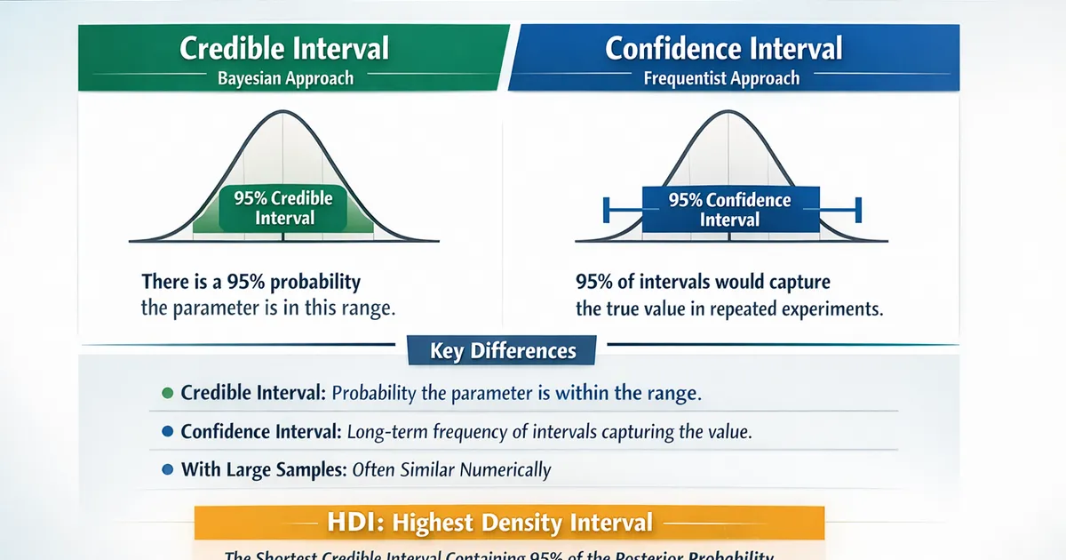
- •A 95% credible interval means: there is a 95% probability the parameter is in this range
- •A 95% confidence interval means: if we repeated the experiment many times, 95% of intervals would contain the true value
- •Credible intervals answer the question people actually ask; confidence intervals answer a hypothetical about repetitions
- •With large samples and uninformative priors, the two intervals are nearly identical numerically
- •Highest Density Intervals (HDI) are the shortest credible intervals and are most useful for skewed posteriors
TL;DR
A 95% credible interval says: "There is a 95% probability the true value is in this range." A 95% confidence interval says: "If we repeated this procedure, 95% of intervals would contain the true value." Most people interpret confidence intervals as if they were credible intervals -- but they are not. This guide explains the real difference, when it matters, and how to use each correctly.
The Core Difference
What a Confidence Interval Actually Means
A 95% confidence interval is a property of the procedure, not the specific interval you calculated.
After computing a confidence interval of [2.1%, 5.3%]:
- CORRECT: "If we repeated this experiment and recomputed the interval many times, 95% of those intervals would contain the true parameter."
- INCORRECT: "There is a 95% probability that the true parameter is between 2.1% and 5.3%."
The true parameter is fixed. It is either in the interval or it is not. The 95% refers to the long-run frequency of the procedure, not to this particular interval.
What a Credible Interval Actually Means
A 95% credible interval is a property of the posterior distribution for this specific dataset.
After computing a credible interval of [2.0%, 5.4%]:
- CORRECT: "Given the data and our prior, there is a 95% probability the parameter is between 2.0% and 5.4%."
- This is a direct probability statement about the parameter.
Side-by-Side Example
import numpy as np
from scipy import stats

np.random.seed(42)

# Scenario: Estimating conversion rate lift
# True lift: 3% (unknown to us)
# Observed: 50 extra conversions out of 2000 visitors in treatment
# vs 0 extra in control of 2000

successes_c, n_c = 240, 2000   # Control: 12.0%
successes_t, n_t = 300, 2000   # Treatment: 15.0%

# --- FREQUENTIST: Confidence Interval ---
p_c = successes_c / n_c
p_t = successes_t / n_t
diff = p_t - p_c
se = np.sqrt(p_c*(1-p_c)/n_c + p_t*(1-p_t)/n_t)
ci_freq = (diff - 1.96*se, diff + 1.96*se)

print("FREQUENTIST")
print(f"Point estimate: {diff:.1%}")
print(f"95% Confidence Interval: [{ci_freq[0]:.1%}, {ci_freq[1]:.1%}]")
print("Interpretation: If we repeated this experiment many times,")
print("95% of such intervals would contain the true difference.\n")

# --- BAYESIAN: Credible Interval ---
post_c = stats.beta(1 + successes_c, 1 + n_c - successes_c)
post_t = stats.beta(1 + successes_t, 1 + n_t - successes_t)

samples_c = post_c.rvs(100000)
samples_t = post_t.rvs(100000)
diff_samples = samples_t - samples_c

ci_bayes = np.percentile(diff_samples, [2.5, 97.5])

print("BAYESIAN")
print(f"Posterior mean: {np.mean(diff_samples):.1%}")
print(f"95% Credible Interval: [{ci_bayes[0]:.1%}, {ci_bayes[1]:.1%}]")
print("Interpretation: There is a 95% probability the true")
print("difference is in this range, given our data and prior.")
Notice the numbers are similar. The difference is what you can say about them.
Types of Credible Intervals
Equal-Tailed Interval (ETI)
The most common type. It excludes 2.5% of the posterior on each side.
def equal_tailed_interval(samples, level=0.95):
    """Standard equal-tailed credible interval."""
    alpha = 1 - level
    lower = np.percentile(samples, 100 * alpha / 2)
    upper = np.percentile(samples, 100 * (1 - alpha / 2))
    return lower, upper
Best for: Symmetric or near-symmetric posteriors. Simple to compute and explain.
Highest Density Interval (HDI)
The shortest interval that contains 95% of the posterior mass. It includes the most probable values.
def highest_density_interval(samples, level=0.95):
    """
    Shortest interval containing the specified probability mass.
    More informative than ETI for skewed distributions.
    """
    sorted_samples = np.sort(samples)
    n = len(sorted_samples)
    interval_size = int(np.ceil(level * n))

    # Find the shortest interval
    widths = sorted_samples[interval_size:] - sorted_samples[:n - interval_size]
    best_idx = np.argmin(widths)

    return sorted_samples[best_idx], sorted_samples[best_idx + interval_size]
Best for: Skewed posteriors (e.g., variance parameters, rate parameters). The HDI excludes the least probable values, which makes more intuitive sense.
When They Differ
# Skewed distribution example: estimating a rate parameter
np.random.seed(42)
samples = np.random.gamma(3, 2, 100000)  # Right-skewed

eti = equal_tailed_interval(samples)
hdi = highest_density_interval(samples)

print(f"ETI: [{eti[0]:.2f}, {eti[1]:.2f}] width = {eti[1]-eti[0]:.2f}")
print(f"HDI: [{hdi[0]:.2f}, {hdi[1]:.2f}] width = {hdi[1]-hdi[0]:.2f}")
print(f"\nHDI is shorter because it captures the mode region")
print(f"ETI wastes probability mass in the thin right tail")
For symmetric posteriors (e.g., Normal), ETI and HDI are identical.
When the Difference Matters
Case 1: Small Samples
With small samples, confidence intervals can include impossible values (e.g., negative conversion rates). Credible intervals with proper priors stay within sensible bounds.
# Small sample: 3 out of 10 converted
successes, n = 3, 10

# Frequentist CI (Wald)
p_hat = successes / n
se = np.sqrt(p_hat * (1 - p_hat) / n)
ci_freq = (p_hat - 1.96*se, p_hat + 1.96*se)

# Bayesian credible interval (Beta prior)
post = stats.beta(1 + successes, 1 + n - successes)
ci_bayes = post.ppf([0.025, 0.975])

print(f"Frequentist CI: [{ci_freq[0]:.1%}, {ci_freq[1]:.1%}]")
print(f"Bayesian CI:    [{ci_bayes[0]:.1%}, {ci_bayes[1]:.1%}]")
print(f"\nFrequentist CI lower bound is near zero or negative with tiny samples")
print(f"Bayesian CI stays within [0, 1] naturally due to the Beta distribution")
Case 2: Informative Priors
When you have strong prior information, credible intervals are narrower and more accurate. Confidence intervals ignore prior knowledge entirely.
Case 3: Communication to Stakeholders
"There is a 95% probability the lift is between 1% and 5%" is immediately useful for decisions.
"If we repeated this experiment, 95% of intervals would contain the true lift" is technically correct but practically unhelpful for this specific decision.
Common Pitfalls
Pitfall 1: Interpreting Confidence Intervals as Credible Intervals
This is the most common statistical misinterpretation in applied work. If you catch yourself saying "there is a 95% chance the parameter is in this interval" about a confidence interval, you are making a Bayesian claim without doing Bayesian inference.
Pitfall 2: Assuming Credible Intervals Are Always Narrower
Credible intervals with uninformative priors are the same width as confidence intervals. Informative priors can make them narrower, but skeptical or wide priors can make them wider.
Pitfall 3: Ignoring the Prior's Influence
With small samples, the credible interval is heavily influenced by the prior. Always do a sensitivity analysis: does your conclusion change with a different reasonable prior?
Quick Reference
| Feature | Confidence Interval | Credible Interval |
|---|---|---|
| Probability statement about parameter | No | Yes |
| Requires prior | No | Yes |
| Long-run frequency guarantee | Yes | No (not its purpose) |
| Works with small samples | Can be unreliable | Stabilized by prior |
| Handles skewed parameters | Same formula | HDI adapts to shape |
| Computational cost | Low | Low to moderate |
Related Methods
- Bayesian Methods Overview (Pillar) - Full Bayesian framework
- Bayesian vs. Frequentist - Framework comparison
- Prior Selection - How priors affect intervals
- Bayesian A/B Testing - Credible intervals in experiments
Key Takeaway
Credible intervals give you what most people want: a direct probability statement that the parameter lies in a given range. Confidence intervals describe the long-run performance of a procedure, not a probability about the parameter for your specific experiment. In practice, the numbers are often similar, but the interpretation is fundamentally different. Use credible intervals when you want to make direct probability statements about your parameter.
References
- https://doi.org/10.3758/s13423-013-0572-3
- https://doi.org/10.1016/j.jmp.2017.05.006
- https://mc-stan.org/users/documentation/
Frequently Asked Questions
Do credible intervals and confidence intervals give different numbers?
Which interval should I report?
What is a Highest Density Interval (HDI)?
Key Takeaway
Credible intervals give you what most people want: a direct probability statement that the parameter lies in a given range. Confidence intervals describe the long-run performance of a procedure, not a probability about the parameter for your specific experiment. In practice, the numbers are often similar, but the interpretation is fundamentally different. Use credible intervals when you want to make direct probability statements about your parameter.