Contents
Prior Selection: Informative, Weakly Informative, and Uninformative
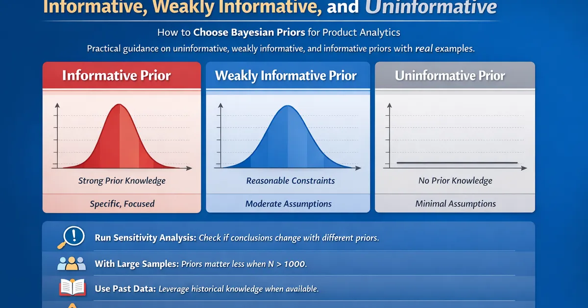
How to choose Bayesian priors for product analytics. Practical guidance on uninformative, weakly informative, and informative priors with real examples.
Quick Hits
- •Uninformative priors let the data speak -- use when you have no prior knowledge
- •Weakly informative priors constrain parameters to sensible ranges -- the recommended default for most product analytics
- •Informative priors encode specific knowledge from past experiments or domain expertise
- •Always run a sensitivity analysis: if your conclusion flips with a different reasonable prior, you need more data
- •With large samples (>1000 per group), the prior barely matters -- the data dominates
TL;DR
Choosing a Bayesian prior is simpler than it sounds. Uninformative priors let the data speak entirely. Weakly informative priors keep estimates in sensible ranges. Informative priors encode real knowledge from past experiments. This guide covers when to use each, how to set them, and how to check whether your choice matters.
The Three Types of Priors
Uninformative (Flat) Priors
What: Assign roughly equal probability to all parameter values.
When: You have no prior knowledge and want results driven entirely by data.
Examples:
- Beta(1, 1) for a proportion -- uniform on [0, 1]
- Normal(0, 10000) for a mean -- effectively flat over any reasonable range
- Improper flat prior on the real line
import numpy as np
from scipy import stats
import matplotlib
matplotlib.use('Agg')

# Uninformative prior for conversion rate
# Beta(1,1) = Uniform(0,1)
prior = stats.beta(1, 1)

# After observing 30 conversions out of 200
posterior = stats.beta(1 + 30, 1 + 200 - 30)

print(f"Prior mean: {prior.mean():.2f} (completely uninformative)")
print(f"Posterior mean: {posterior.mean():.1%}")
print(f"95% CI: [{posterior.ppf(0.025):.1%}, {posterior.ppf(0.975):.1%}]")
Trade-off: With small samples, uninformative priors can produce unstable or extreme estimates. For example, 0 out of 5 users converting gives a posterior mean near 0%, ignoring the reality that the true rate is unlikely to be exactly zero.
Weakly Informative Priors
What: Constrain parameters to plausible ranges without committing to specific values. The recommended default for most analyses.
When: You know the general scale of the parameter but not its precise value.
Examples:
- Beta(2, 20) for a conversion rate you expect to be around 5-15%
- Normal(0, 1) for a standardized effect size
- Half-Normal(0, 10) for a standard deviation
# Weakly informative prior for conversion rate
# We know rates are typically 5-20% for this product
# Beta(2, 18) has mean ~10%, spread covers 2-25%
prior_weak = stats.beta(2, 18)

# After observing 30 conversions out of 200
posterior_weak = stats.beta(2 + 30, 18 + 200 - 30)

# Compare with uninformative
posterior_flat = stats.beta(1 + 30, 1 + 200 - 30)

print("Weakly informative prior:")
print(f"  Prior mean: {prior_weak.mean():.1%}")
print(f"  Posterior mean: {posterior_weak.mean():.1%}")
print(f"  95% CI: [{posterior_weak.ppf(0.025):.1%}, {posterior_weak.ppf(0.975):.1%}]")
print(f"\nUninformative prior:")
print(f"  Posterior mean: {posterior_flat.mean():.1%}")
print(f"  95% CI: [{posterior_flat.ppf(0.025):.1%}, {posterior_flat.ppf(0.975):.1%}]")
print(f"\nDifference is small with n=200. With n=20 it would be larger.")
Why this is the default recommendation: Weakly informative priors prevent pathological estimates (like a conversion rate of 0% or 100%) while having minimal influence when you have reasonable amounts of data.
Informative Priors
What: Encode specific knowledge -- usually from past experiments, historical data, or published research.
When: You have strong, quantitative prior knowledge relevant to the current analysis.
Examples:
- Beta(120, 880) for a conversion rate if past data shows 12% with 1000 observations
- Normal(0.03, 0.02) for a treatment effect if past experiments show 3% lifts with 2% SD
# Informative prior from past experiments
# Last 10 experiments showed a mean conversion rate of 12%
# with about 1000 total observations equivalent
prior_info = stats.beta(120, 880)  # Mean ~12%, tight

# Current experiment: 30 out of 200
posterior_info = stats.beta(120 + 30, 880 + 200 - 30)

print("Informative prior (from historical data):")
print(f"  Prior mean: {prior_info.mean():.1%}")
print(f"  Prior 95% CI: [{prior_info.ppf(0.025):.1%}, {prior_info.ppf(0.975):.1%}]")
print(f"  Posterior mean: {posterior_info.mean():.1%}")
print(f"  Posterior 95% CI: [{posterior_info.ppf(0.025):.1%}, {posterior_info.ppf(0.975):.1%}]")
print(f"\nNote: With only 200 new observations, the informative prior")
print(f"(equivalent to 1000 observations) heavily influences the posterior.")
print(f"The posterior is pulled toward the prior mean of 12%.")
Caution: Informative priors carry strong assumptions. If the current situation differs from the historical data (new market, different user segment, product redesign), the prior may be misleading.
How to Set Priors in Practice
Step 1: Identify the Parameter Type
| Parameter | Common Prior | Notes |
|---|---|---|
| Proportion (0 to 1) | Beta(a, b) | a, b control mean and concentration |
| Mean (continuous) | Normal(mu, sigma) | mu = center, sigma = uncertainty |
| Standard deviation | Half-Normal(0, s) or Exponential(rate) | Must be positive |
| Count | Poisson(lambda) or Gamma(a, b) | Must be non-negative |
| Regression coefficient | Normal(0, s) | s controls regularization strength |
Step 2: Translate Knowledge to Parameters
For a Beta prior on a conversion rate:
- Expected rate ~10%: Set mean = a/(a+b) = 0.10
- How confident? a + b controls concentration (higher = more confident)
- a + b = 2: Very uncertain (almost flat)
- a + b = 20: Moderate confidence
- a + b = 200: Strong confidence (equivalent to 200 prior observations)
def beta_from_mean_sample_size(mean, sample_size):
    """
    Create Beta prior from mean and effective sample size.

    mean: expected proportion (0-1)
    sample_size: effective prior observations (higher = more confident)
    """
    alpha = mean * sample_size
    beta = (1 - mean) * sample_size
    prior = stats.beta(alpha, beta)
    return {
        'alpha': alpha,
        'beta': beta,
        'mean': prior.mean(),
        'ci_95': (prior.ppf(0.025), prior.ppf(0.975))
    }

# "I think the conversion rate is around 10%, but I'm not very sure"
prior = beta_from_mean_sample_size(0.10, 10)
print(f"Prior: Beta({prior['alpha']:.1f}, {prior['beta']:.1f})")
print(f"Mean: {prior['mean']:.1%}, 95% range: [{prior['ci_95'][0]:.1%}, {prior['ci_95'][1]:.1%}]")
Step 3: Prior Predictive Check
Before seeing data, simulate from your prior and see if the predictions make sense:
def prior_predictive_check(prior_alpha, prior_beta, n_trials=1000, n_simulations=5000):
    """
    Simulate data from the prior to check if the prior is sensible.
    """
    # Draw conversion rates from prior
    rates = stats.beta(prior_alpha, prior_beta).rvs(n_simulations)

    # Simulate observed conversions
    conversions = np.random.binomial(n_trials, rates)

    print("Prior Predictive Check")
    print(f"Prior: Beta({prior_alpha}, {prior_beta})")
    print(f"Simulated {n_simulations} datasets with n={n_trials}")
    print(f"Conversion rate range: [{np.percentile(rates, 2.5):.1%}, {np.percentile(rates, 97.5):.1%}]")
    print(f"Conversions range: [{np.percentile(conversions, 2.5):.0f}, {np.percentile(conversions, 97.5):.0f}]")
    print(f"\nDo these ranges look reasonable for your product?")

prior_predictive_check(2, 18)  # Weakly informative
Sensitivity Analysis
The most important step in any Bayesian analysis. Does your conclusion change with different priors?
def prior_sensitivity(successes, trials, priors_dict):
    """
    Check how posterior changes across different priors.
    """
    print(f"Data: {successes}/{trials} = {successes/trials:.1%}")
    print(f"{'Prior':<30} {'Posterior Mean':<18} {'95% CI':<25} {'P(rate>10%)'}")
    print("-" * 90)

    for name, (a, b) in priors_dict.items():
        post = stats.beta(a + successes, b + trials - successes)
        samples = post.rvs(50000)
        ci = post.ppf([0.025, 0.975])
        p_above = np.mean(samples > 0.10)
        print(f"{name:<30} {post.mean():<18.1%} [{ci[0]:.1%}, {ci[1]:.1%}]{'':<5} {p_above:.1%}")


prior_sensitivity(25, 200, {
    'Flat: Beta(1,1)': (1, 1),
    'Weakly informative: Beta(2,18)': (2, 18),
    'Informative (12%): Beta(12,88)': (12, 88),
    'Strong (12%): Beta(120,880)': (120, 880),
    'Skeptical (5%): Beta(5,95)': (5, 95),
})
If all priors give the same conclusion, your result is robust. If they disagree, you need more data.
Recommendations by Scenario
| Scenario | Recommended Prior | Why |
|---|---|---|
| Standard A/B test, large sample | Uninformative Beta(1,1) | Data dominates; keep it simple |
| A/B test, small sample (<500) | Weakly informative | Prevents extreme estimates |
| Sequential experiment | Weakly informative | Stabilizes early estimates |
| Known baseline rate | Informative (from historical) | Leverages existing knowledge |
| Multi-arm bandit | Informative from past arms | Speeds up learning |
| Regression coefficients | Normal(0, s) weakly informative | Provides regularization |
Related Methods
- Bayesian Methods Overview (Pillar) - Complete Bayesian framework
- Credible Intervals - How priors affect intervals
- Bayesian A/B Testing - Priors in experiments
- Bayesian Regression - Priors as regularization
- Bayesian Sample Size - Prior influence on planning
Key Takeaway
For most product analytics, weakly informative priors are the best default. They prevent absurd estimates without imposing strong assumptions. Use uninformative priors when you want results equivalent to frequentist analysis. Use informative priors when you have strong historical data. Always run a sensitivity analysis to check whether your conclusions depend on the prior choice.
References
- https://doi.org/10.1214/08-AOS595
- https://mc-stan.org/users/documentation/case-studies/weakly_informative_priors.html
- https://github.com/stan-dev/stan/wiki/Prior-Choice-Recommendations
Frequently Asked Questions
What if I choose the wrong prior?
Are uninformative priors truly uninformative?
Can I use data from the current experiment to choose the prior?
Key Takeaway
For most product analytics, weakly informative priors are the best default. They prevent absurd estimates without imposing strong assumptions. Use uninformative priors when you want results equivalent to frequentist analysis. Use informative priors when you have strong historical data. Always run a sensitivity analysis to check whether your conclusions depend on the prior choice.