Contents
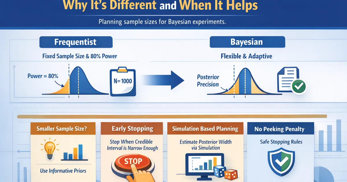
Bayesian Sample Size: Why It's Different and When It Helps
How to plan sample sizes for Bayesian experiments. Learn why Bayesian sample sizing differs from frequentist, and when it gives you smaller or more flexible experiments.
Quick Hits
- •Bayesian experiments do not require a fixed sample size -- but you still need enough data for useful conclusions
- •Instead of power, think posterior precision: how narrow does your credible interval need to be?
- •Informative priors effectively add 'free' observations, reducing the data you need to collect
- •Simulation-based planning lets you estimate how many observations you need for a given posterior width
- •Bayesian stopping rules do not inflate error rates, unlike peeking in frequentist tests
TL;DR
Bayesian experiments do not require a fixed sample size determined by power analysis. Instead, you plan based on posterior precision: how many observations do you need for a credible interval narrow enough to make a decision? This guide covers simulation-based planning, the role of priors in sample size, and when Bayesian flexibility actually helps.
Why Bayesian Sample Size Is Different
Frequentist: Fixed Sample, Binary Outcome
Frequentist power analysis asks: "How many observations do I need to have an 80% chance of detecting a 2% effect at alpha = 0.05?"
This gives you a fixed number. You must collect exactly that many observations. Stopping early inflates your false positive rate. Stopping late wastes resources.
Bayesian: Flexible Sample, Continuous Monitoring
Bayesian planning asks: "How many observations do I need for my posterior to be precise enough to make a confident decision?"
There is no single magic number. You can check the posterior at any time. The posterior is always valid -- it just gets more precise as you collect more data.
import numpy as np
from scipy import stats

def posterior_width_by_sample_size(true_rate=0.12, effect=0.02,
                                    sample_sizes=[100, 250, 500, 1000, 2500, 5000],
                                    prior_a=1, prior_b=1, n_simulations=500):
    """
    Simulate posterior width as a function of sample size.
    """
    print(f"True control rate: {true_rate:.1%}")
    print(f"True effect: {effect:.1%}")
    print(f"Prior: Beta({prior_a}, {prior_b})")
    print(f"\n{'n per arm':<12} {'Median CI Width':<18} {'P(detect effect)':<20} {'Median P(B>A)'}")
    print("-" * 70)

    for n in sample_sizes:
        ci_widths = []
        detected = 0
        p_better_list = []

        for _ in range(n_simulations):
            # Simulate data
            control_conv = np.random.binomial(n, true_rate)
            treatment_conv = np.random.binomial(n, true_rate + effect)

            # Posterior samples
            c_post = stats.beta(prior_a + control_conv, prior_b + n - control_conv)
            t_post = stats.beta(prior_a + treatment_conv, prior_b + n - treatment_conv)

            c_samples = c_post.rvs(10000)
            t_samples = t_post.rvs(10000)
            diff = t_samples - c_samples

            # Metrics
            ci = np.percentile(diff, [2.5, 97.5])
            ci_widths.append(ci[1] - ci[0])
            p_better = np.mean(diff > 0)
            p_better_list.append(p_better)
            if p_better > 0.95:
                detected += 1

        median_width = np.median(ci_widths)
        detection_rate = detected / n_simulations
        median_p = np.median(p_better_list)

        print(f"{n:<12} {median_width:<18.4f} {detection_rate:<20.1%} {median_p:.1%}")


posterior_width_by_sample_size()
Simulation-Based Sample Size Planning
The Core Approach
- Define the minimum effect size you care about
- Choose your prior
- Set your decision criterion (e.g., 95% credible interval excludes zero, or P(better) > 95%)
- Simulate experiments at various sample sizes
- Find the smallest n where your criterion is met most of the time
def bayesian_sample_size(target_effect=0.02, base_rate=0.12,
                          desired_precision=0.02, confidence=0.80,
                          prior_a=1, prior_b=1, n_simulations=1000):
    """
    Find sample size for desired posterior precision.

    desired_precision: maximum 95% CI width you'll accept
    confidence: proportion of simulations that should achieve the precision
    """
    for n in [50, 100, 200, 500, 1000, 2000, 5000, 10000]:
        precise_count = 0

        for _ in range(n_simulations):
            control_conv = np.random.binomial(n, base_rate)
            treatment_conv = np.random.binomial(n, base_rate + target_effect)

            c_samples = stats.beta(prior_a + control_conv, prior_b + n - control_conv).rvs(5000)
            t_samples = stats.beta(prior_a + treatment_conv, prior_b + n - treatment_conv).rvs(5000)
            diff = t_samples - c_samples

            ci_width = np.percentile(diff, 97.5) - np.percentile(diff, 2.5)
            if ci_width <= desired_precision:
                precise_count += 1

        prop_precise = precise_count / n_simulations
        if prop_precise >= confidence:
            print(f"Recommended: n = {n} per arm")
            print(f"  {prop_precise:.0%} of simulations achieve CI width <= {desired_precision}")
            return n

    print("Need more than 10,000 per arm")
    return None


recommended_n = bayesian_sample_size(
    target_effect=0.02,
    base_rate=0.12,
    desired_precision=0.03,
    confidence=0.80
)
How Priors Affect Sample Size
Informative Priors as "Free Data"
An informative prior is mathematically equivalent to having already observed data. A Beta(12, 88) prior on a conversion rate acts like 100 prior observations with a 12% rate.
def prior_impact_on_sample_size(true_rate=0.12, effect=0.02,
                                 priors={'Flat Beta(1,1)': (1, 1),
                                         'Weak Beta(2,18)': (2, 18),
                                         'Informative Beta(12,88)': (12, 88)},
                                 threshold_prob=0.95,
                                 n_simulations=500):
    """
    Show how different priors affect required sample size.
    """
    print(f"Effect to detect: {effect:.1%}")
    print(f"Decision criterion: P(B > A) > {threshold_prob:.0%}")
    print(f"\n{'Prior':<30} {'n=200':<12} {'n=500':<12} {'n=1000':<12} {'n=2000'}")
    print("-" * 70)

    for prior_name, (a, b) in priors.items():
        results = []
        for n in [200, 500, 1000, 2000]:
            detected = 0
            for _ in range(n_simulations):
                cc = np.random.binomial(n, true_rate)
                tc = np.random.binomial(n, true_rate + effect)

                c_s = stats.beta(a + cc, b + n - cc).rvs(5000)
                t_s = stats.beta(a + tc, b + n - tc).rvs(5000)
                p_better = np.mean(t_s > c_s)
                if p_better > threshold_prob:
                    detected += 1
            results.append(f"{detected/n_simulations:.0%}")

        print(f"{prior_name:<30} {'  '.join(f'{r:<12}' for r in results)}")


prior_impact_on_sample_size()
Informative priors reduce the sample needed -- but only if the prior accurately reflects reality. A wrong informative prior can slow convergence to the truth.
Bayesian Stopping Rules
Why You Can Peek
In frequentist testing, peeking inflates the false positive rate because each look is an opportunity to stop when noise looks like signal.
Bayesian inference does not have this problem. The posterior at any point is a valid summary of what you know given the data so far. There is no "multiple testing" penalty.
Practical Stopping Criteria
def monitor_experiment(control_stream, treatment_stream,
                       min_per_arm=100, max_per_arm=10000,
                       loss_threshold=0.0005, check_every=50):
    """
    Monitor a Bayesian experiment with stopping rules.
    """
    c_successes, c_total = 0, 0
    t_successes, t_total = 0, 0

    for i in range(max_per_arm):
        # Accumulate data
        c_successes += control_stream[i]
        c_total += 1
        t_successes += treatment_stream[i]
        t_total += 1

        # Check at intervals
        if c_total >= min_per_arm and c_total % check_every == 0:
            c_samples = stats.beta(1 + c_successes, 1 + c_total - c_successes).rvs(10000)
            t_samples = stats.beta(1 + t_successes, 1 + t_total - t_successes).rvs(10000)
            diff = t_samples - c_samples

            loss_ship = np.mean(np.maximum(-diff, 0))
            loss_hold = np.mean(np.maximum(diff, 0))
            p_better = np.mean(diff > 0)

            if loss_ship < loss_threshold:
                return {
                    'decision': 'Ship',
                    'n_per_arm': c_total,
                    'p_better': p_better,
                    'expected_loss': loss_ship
                }
            if loss_hold < loss_threshold:
                return {
                    'decision': 'Hold (control is better)',
                    'n_per_arm': c_total,
                    'p_better': p_better,
                    'expected_loss': loss_hold
                }

    return {'decision': 'Inconclusive', 'n_per_arm': max_per_arm}


# Simulate data stream
np.random.seed(42)
control = np.random.binomial(1, 0.12, 10000)
treatment = np.random.binomial(1, 0.14, 10000)

result = monitor_experiment(control, treatment)
print(f"Decision: {result['decision']} at n={result['n_per_arm']} per arm")
print(f"P(Treatment better): {result.get('p_better', 'N/A'):.1%}")
Comparison with Frequentist Planning
| Aspect | Frequentist Power Analysis | Bayesian Planning |
|---|---|---|
| Goal | Detect effect at given power/alpha | Achieve desired posterior precision |
| Output | Fixed sample size | Range or minimum sample size |
| Stopping | Fixed (or sequential with correction) | Flexible (check anytime) |
| Priors | Not used | Reduce required sample size |
| Computation | Closed-form formulas | Simulation-based |
| Peeking | Inflates false positive rate | No inflation |
Practical Recommendations
-
Always set a minimum sample size: Even with Bayesian methods, tiny samples produce posteriors dominated by the prior. Aim for at least 100 events (conversions, clicks) per variant.
-
Use simulation for planning: There is no simple formula. Simulate data under your expected effect, compute posteriors, and find the sample size that gives you useful precision.
-
Include priors in planning: If you have informative priors, factor them in. They reduce the data you need.
-
Set a maximum duration: Experiments that run forever waste traffic. Set a calendar deadline even if using flexible stopping.
Related Methods
- Bayesian Methods Overview (Pillar) - Full Bayesian framework
- Bayesian A/B Testing - Running the experiment
- Prior Selection - Priors affect sample size
- Bayesian vs. Frequentist - Comparing planning approaches
Key Takeaway
Bayesian sample size planning focuses on posterior precision rather than frequentist power. You ask "How many observations until my credible interval is narrow enough to make a decision?" instead of "How many observations to achieve 80% power?" This approach is more flexible, allows early stopping without error inflation, and naturally incorporates prior information. Use simulation to plan: generate datasets under your expected effect, compute posteriors, and find the sample size where the posterior is precise enough for your decision.
References
- https://doi.org/10.1080/00031305.2018.1564697
- https://doi.org/10.3758/s13423-015-0947-8
- https://mc-stan.org/users/documentation/
Frequently Asked Questions
Does Bayesian testing require fewer samples?
How do I do a power analysis for a Bayesian test?
Can I just run the experiment and stop whenever the posterior looks good?
Key Takeaway
Bayesian sample size planning focuses on posterior precision rather than frequentist power. You ask 'How many observations until my credible interval is narrow enough to make a decision?' instead of 'How many observations to achieve 80% power?' This approach is more flexible, allows early stopping without error inflation, and naturally incorporates prior information. Use simulation to plan: generate datasets under your expected effect, compute posteriors, and find the sample size where the posterior is precise enough for your decision.