Contents
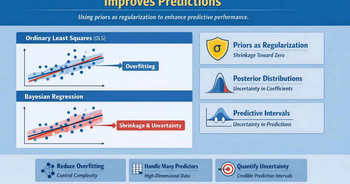
Bayesian Regression: When Shrinkage Improves Predictions
Learn how Bayesian regression uses priors as regularization to improve predictions. Practical guide to shrinkage, uncertainty quantification, and when it beats OLS.
Quick Hits
- •Bayesian regression priors act as regularization -- a Normal(0, sigma) prior on coefficients is mathematically equivalent to ridge regression
- •You get a full posterior distribution for every coefficient, not just a point estimate and standard error
- •Posterior predictive distributions give you uncertainty on predictions, not just the mean
- •Shrinkage toward zero reduces overfitting, especially with many predictors or correlated features
- •Bayesian regression shines when you have more features than observations or need honest uncertainty quantification
TL;DR
Bayesian regression adds priors to regression coefficients, which acts as regularization (shrinkage). A Normal prior on coefficients is equivalent to ridge regression, but you also get full uncertainty quantification. This guide covers when shrinkage improves predictions, how to set priors on regression coefficients, and how to use posterior predictive distributions for honest prediction intervals.
Why Bayesian Regression
The OLS Problem
Ordinary Least Squares (OLS) regression finds the coefficients that minimize squared error. It works well with lots of data and few predictors. But it fails when:
- Many predictors: Coefficients overfit noise, predictions are poor on new data
- Correlated features: Coefficient estimates are unstable and have large standard errors
- Small samples: Not enough data to estimate all coefficients reliably
- Uncertainty needed: OLS gives point predictions, not prediction intervals
The Bayesian Solution
Bayesian regression adds prior distributions to coefficients. These priors:
- Shrink estimates toward zero (or toward a prior mean), reducing overfitting
- Stabilize correlated coefficient estimates
- Provide full posterior distributions for coefficients and predictions
Bayesian Linear Regression
The Model
With priors:
Implementation
import numpy as np
from scipy import stats

def bayesian_linear_regression(X, y, prior_var=1.0):
    """
    Bayesian linear regression with Normal prior.
    Conjugate solution (no MCMC needed for linear case).

    prior_var: variance of Normal(0, prior_var) prior on coefficients
    """
    n, p = X.shape

    # OLS estimate for comparison
    beta_ols = np.linalg.lstsq(X, y, rcond=None)[0]
    residuals = y - X @ beta_ols
    sigma2_hat = np.sum(residuals**2) / (n - p)

    # Bayesian posterior (conjugate Normal-Normal)
    prior_precision = np.eye(p) / prior_var
    data_precision = X.T @ X / sigma2_hat
    posterior_precision = prior_precision + data_precision
    posterior_cov = np.linalg.inv(posterior_precision)
    posterior_mean = posterior_cov @ (X.T @ y / sigma2_hat)

    return {
        'beta_ols': beta_ols,
        'beta_bayes': posterior_mean,
        'posterior_cov': posterior_cov,
        'posterior_sd': np.sqrt(np.diag(posterior_cov)),
        'sigma2_hat': sigma2_hat,
        'shrinkage': 1 - np.linalg.norm(posterior_mean) / np.linalg.norm(beta_ols)
    }


# Example: predicting revenue per user
np.random.seed(42)
n = 100
p = 10

# Features: user behavior metrics
X = np.random.randn(n, p)
X[:, 3] = X[:, 0] + np.random.randn(n) * 0.3  # Correlated features

# True coefficients (only 3 are non-zero)
true_beta = np.zeros(p)
true_beta[0] = 2.0
true_beta[1] = -1.5
true_beta[2] = 1.0

y = X @ true_beta + np.random.randn(n) * 2

result = bayesian_linear_regression(X, y, prior_var=5.0)

print("Coefficient Comparison")
print(f"{'Feature':<10} {'True':<10} {'OLS':<10} {'Bayes':<10} {'Post SD'}")
print("-" * 55)
for j in range(p):
    print(f"x{j:<9} {true_beta[j]:<10.2f} {result['beta_ols'][j]:<10.2f} "
          f"{result['beta_bayes'][j]:<10.2f} {result['posterior_sd'][j]:.2f}")

print(f"\nShrinkage: {result['shrinkage']:.1%} of coefficients shrunk toward zero")
Shrinkage as Regularization
Normal Prior = Ridge Regression
A Normal(0, tau^2) prior on coefficients penalizes large values, just like ridge regression's L2 penalty:
| Bayesian | Frequentist Equivalent |
|---|---|
| Normal(0, tau^2) prior | Ridge regression (lambda = sigma^2/tau^2) |
| Laplace(0, b) prior | Lasso regression (lambda = sigma^2/b) |
| Horseshoe prior | Adaptive shrinkage (sparse models) |
The Bayesian approach is more flexible because you can use different priors for different coefficients.
When Shrinkage Helps
def compare_ols_vs_bayesian(n_train=50, n_test=200, p=20, n_true=5,
                              prior_vars=[0.1, 1.0, 10.0, 100.0],
                              n_simulations=200):
    """
    Compare prediction error of OLS vs. Bayesian regression.
    """
    results = {'OLS': []}
    for pv in prior_vars:
        results[f'Bayes(var={pv})'] = []

    for _ in range(n_simulations):
        X_train = np.random.randn(n_train, p)
        X_test = np.random.randn(n_test, p)

        true_beta = np.zeros(p)
        true_beta[:n_true] = np.random.randn(n_true)

        y_train = X_train @ true_beta + np.random.randn(n_train)
        y_test = X_test @ true_beta + np.random.randn(n_test)

        # OLS
        try:
            beta_ols = np.linalg.lstsq(X_train, y_train, rcond=None)[0]
            mse_ols = np.mean((y_test - X_test @ beta_ols)**2)
            results['OLS'].append(mse_ols)
        except np.linalg.LinAlgError:
            results['OLS'].append(np.nan)

        # Bayesian with different prior variances
        for pv in prior_vars:
            sigma2 = np.var(y_train - X_train.mean(axis=0) @ np.zeros(p))
            prior_prec = np.eye(p) / pv
            post_prec = prior_prec + X_train.T @ X_train / sigma2
            post_cov = np.linalg.inv(post_prec)
            beta_bayes = post_cov @ (X_train.T @ y_train / sigma2)
            mse_bayes = np.mean((y_test - X_test @ beta_bayes)**2)
            results[f'Bayes(var={pv})'].append(mse_bayes)

    print(f"Test MSE (n_train={n_train}, p={p}, {n_true} true features)")
    print("-" * 50)
    for name, mses in results.items():
        print(f"{name:<20} Mean MSE: {np.nanmean(mses):.3f}")


compare_ols_vs_bayesian()
With many predictors relative to observations, Bayesian shrinkage consistently beats OLS on test data.
Posterior Predictive Distributions
Uncertainty on Predictions
OLS gives you a single predicted value. Bayesian regression gives you a full distribution:
def posterior_predictive(X_new, X_train, y_train, prior_var=5.0):
    """
    Posterior predictive distribution for new data points.
    Returns mean and credible intervals for predictions.
    """
    n, p = X_train.shape

    # Fit posterior
    sigma2_hat = np.var(y_train - X_train @ np.linalg.lstsq(X_train, y_train, rcond=None)[0])

    prior_prec = np.eye(p) / prior_var
    post_prec = prior_prec + X_train.T @ X_train / sigma2_hat
    post_cov = np.linalg.inv(post_prec)
    post_mean = post_cov @ (X_train.T @ y_train / sigma2_hat)

    # Predictive distribution
    pred_mean = X_new @ post_mean
    pred_var = np.array([
        x @ post_cov @ x + sigma2_hat  # uncertainty in beta + noise
        for x in X_new
    ])
    pred_sd = np.sqrt(pred_var)

    return {
        'mean': pred_mean,
        'lower_95': pred_mean - 1.96 * pred_sd,
        'upper_95': pred_mean + 1.96 * pred_sd,
        'sd': pred_sd
    }


# New users to predict
X_new = np.random.randn(5, p)
preds = posterior_predictive(X_new, X, y, prior_var=5.0)

print("Predictions with Uncertainty")
print(f"{'User':<8} {'Predicted':<12} {'95% Interval':<25}")
print("-" * 45)
for i in range(5):
    print(f"User {i+1:<3} {preds['mean'][i]:<12.2f} "
          f"[{preds['lower_95'][i]:.2f}, {preds['upper_95'][i]:.2f}]")
These prediction intervals honestly account for both parameter uncertainty and observation noise. OLS prediction intervals often underestimate uncertainty, especially with many predictors.
Choosing Priors for Regression
Default Recommendations
| Coefficient Type | Recommended Prior | Why |
|---|---|---|
| Standardized features | Normal(0, 1) | Weakly informative, allows moderate effects |
| Raw features | Normal(0, s) where s matches scale | Scale-appropriate shrinkage |
| Intercept | Normal(y_bar, 10*s_y) | Centered at outcome mean, wide |
| Variance (sigma) | Half-Normal(0, s_y) | Weakly informative on scale |
Scaling Matters
Always standardize features before setting priors, or scale priors to match the feature scale. A Normal(0, 1) prior means very different things for a feature in [0, 1] vs. [0, 1000000].
When to Use Bayesian Regression
- Many predictors relative to observations: Shrinkage prevents overfitting
- Prediction intervals needed: Posterior predictive distributions give honest uncertainty
- Correlated features: Priors stabilize unstable coefficient estimates
- Prior knowledge about coefficients: Encode domain expertise directly
- Hierarchical structure: Group-level and individual-level effects (see Hierarchical Models)
Related Methods
- Bayesian Methods Overview (Pillar) - Full framework
- Hierarchical Models - Regression across segments
- Prior Selection - Choosing coefficient priors
- Practical Bayes Tools - brms makes Bayesian regression easy
Key Takeaway
Bayesian regression uses priors as principled regularization. Normal priors on coefficients shrink estimates toward zero, reducing overfitting. Unlike ridge or lasso regression, Bayesian regression gives you full posterior distributions for coefficients and predictions, so you can quantify uncertainty honestly. Use it when you have many predictors, correlated features, small samples, or when stakeholders need prediction intervals rather than point estimates.
References
- https://doi.org/10.1214/10-BA607
- https://mc-stan.org/users/documentation/
- https://paul-buerkner.github.io/brms/
Frequently Asked Questions
Is Bayesian regression the same as ridge regression?
When does Bayesian regression outperform OLS?
Do I need MCMC for Bayesian regression?
Key Takeaway
Bayesian regression uses priors as principled regularization. Normal priors on coefficients shrink estimates toward zero, reducing overfitting. Unlike ridge or lasso regression, Bayesian regression gives you full posterior distributions for coefficients and predictions, so you can quantify uncertainty honestly. Use it when you have many predictors, correlated features, small samples, or when stakeholders need prediction intervals rather than point estimates.