Contents
Practical Bayes: Using PyMC, Stan, and brms for Real Analysis
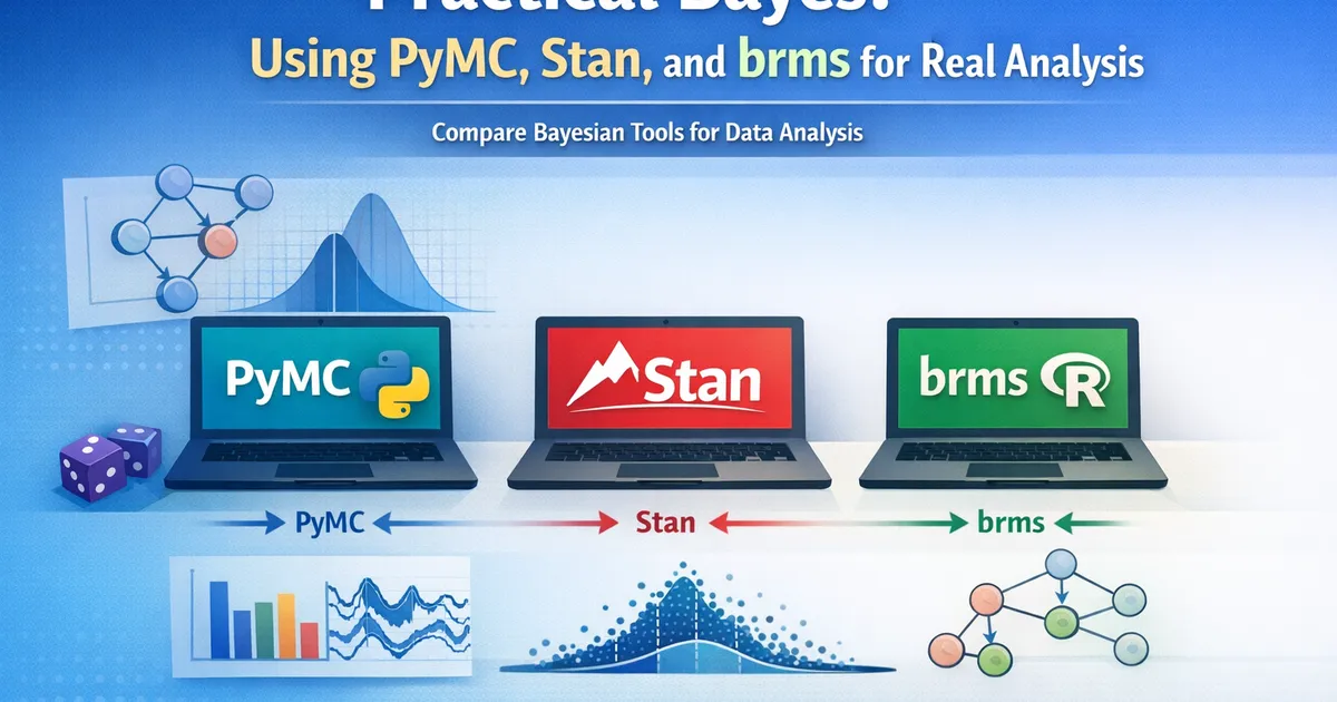
Hands-on guide to Bayesian tools. Compare PyMC, Stan, and brms with real examples. Learn which tool fits your workflow and how to get started fast.
Quick Hits
- •PyMC (Python): Best for custom models, deep integration with the Python data science stack
- •Stan (multi-language): Best for complex hierarchical models and production-grade MCMC performance
- •brms (R): Best for analysts familiar with R's formula syntax -- the fastest path from lm() to Bayesian
- •All three tools use MCMC sampling -- the concepts transfer across tools
- •Start with brms or PyMC for typical product analytics; move to Stan for custom or performance-critical models
TL;DR
Three tools dominate modern Bayesian analysis: PyMC (Python), Stan (multi-language), and brms (R). This guide shows you how to fit the same model in all three, compares their strengths and weaknesses, and helps you choose the right tool for your workflow. All three are production-ready and can handle typical product analytics problems.
Tool Comparison at a Glance
| Feature | PyMC | Stan | brms |
|---|---|---|---|
| Language | Python | C++ (R/Python/etc. interfaces) | R |
| Learning curve | Moderate | Steep | Gentle |
| Model flexibility | High | Very high | Moderate (formula-based) |
| MCMC sampler | NUTS (JAX/NumPyro backend) | NUTS (best-in-class) | Uses Stan backend |
| Speed | Fast | Fastest | Fast (via Stan) |
| Diagnostics | Built-in (ArviZ) | Built-in + ShinyStan | Built-in |
| Custom models | Full control | Full control | Limited to formula syntax |
| Community | Large, growing | Large, established | Large, R-focused |
| Best for | Python data scientists | Complex/custom models | R analysts transitioning to Bayes |
The Same Model in Three Tools
The Problem
You want to estimate the effect of a new checkout flow on conversion rate, controlling for user segment (new vs. returning).
Model: Logistic regression with treatment indicator and user segment.
PyMC (Python)
import pymc as pm
import numpy as np
import arviz as az

# Simulate data
np.random.seed(42)
n = 5000
treatment = np.random.binomial(1, 0.5, n)
returning = np.random.binomial(1, 0.4, n)
logit_p = -2.0 + 0.3 * treatment + 0.5 * returning
p = 1 / (1 + np.exp(-logit_p))
converted = np.random.binomial(1, p, n)

# Model
with pm.Model() as checkout_model:
    # Priors
    beta_0 = pm.Normal('intercept', mu=0, sigma=2)
    beta_treatment = pm.Normal('treatment_effect', mu=0, sigma=1)
    beta_returning = pm.Normal('returning_effect', mu=0, sigma=1)

    # Linear predictor
    logit_p = beta_0 + beta_treatment * treatment + beta_returning * returning

    # Likelihood
    y = pm.Bernoulli('converted', logit_p=logit_p, observed=converted)

    # Sample
    trace = pm.sample(2000, tune=1000, cores=4, random_seed=42)

# Results
summary = az.summary(trace, var_names=['intercept', 'treatment_effect', 'returning_effect'])
print(summary)

# Probability treatment is positive
treatment_samples = trace.posterior['treatment_effect'].values.flatten()
print(f"\nP(treatment effect > 0): {np.mean(treatment_samples > 0):.1%}")
Strengths: Pythonic API, integrates with pandas/numpy/matplotlib, ArviZ for diagnostics.
Stan (via PyStan or CmdStanPy)
// checkout_model.stan
data {
  int<lower=0> N;
  array[N] int<lower=0,upper=1> converted;
  vector[N] treatment;
  vector[N] returning;
}

parameters {
  real intercept;
  real treatment_effect;
  real returning_effect;
}

model {
  // Priors
  intercept ~ normal(0, 2);
  treatment_effect ~ normal(0, 1);
  returning_effect ~ normal(0, 1);

  // Likelihood
  converted ~ bernoulli_logit(intercept +
                               treatment_effect * treatment +
                               returning_effect * returning);
}

generated quantities {
  real prob_treatment_positive = treatment_effect > 0 ? 1 : 0;
}
# Python interface (CmdStanPy)
from cmdstanpy import CmdStanModel

model = CmdStanModel(stan_file='checkout_model.stan')
data = {
    'N': n,
    'converted': converted.tolist(),
    'treatment': treatment.tolist(),
    'returning': returning.tolist()
}
fit = model.sample(data=data, chains=4, iter_sampling=2000, iter_warmup=1000)
print(fit.summary())
Strengths: Fastest sampler, best for complex custom models, excellent diagnostics.
brms (R)
library(brms)

# Data
set.seed(42)
n <- 5000
df <- data.frame(
  treatment = rbinom(n, 1, 0.5),
  returning = rbinom(n, 1, 0.4)
)
df$p <- plogis(-2.0 + 0.3 * df$treatment + 0.5 * df$returning)
df$converted <- rbinom(n, 1, df$p)

# Model (looks just like glm!)
fit <- brm(
  converted ~ treatment + returning,
  data = df,
  family = bernoulli(link = "logit"),
  prior = c(
    prior(normal(0, 2), class = "Intercept"),
    prior(normal(0, 1), class = "b")
  ),
  chains = 4,
  iter = 3000,
  warmup = 1000,
  seed = 42
)

# Results
summary(fit)

# Probability treatment is positive
posterior <- as_draws_df(fit)
cat("P(treatment > 0):", mean(posterior$b_treatment > 0), "\n")
Strengths: Formula syntax identical to glm(), easiest transition for R users, powerful built-in plot functions.
Choosing Your Tool
Decision Framework
Are you a Python user?
├── Yes
│   ├── Standard models (regression, A/B tests)?
│   │   └── PyMC (easiest Python option)
│   └── Custom or complex models?
│       ├── PyMC can express it → PyMC
│       └── Need maximum performance → Stan (via CmdStanPy)
└── No (R user)
    ├── Standard models?
    │   └── brms (formula syntax, fastest setup)
    └── Custom models brms cannot express?
        └── Stan (via RStan or CmdStanR)
When Each Tool Shines
PyMC is best when:
- You work in Python and want to stay in one ecosystem
- You need custom model components (mixture models, custom likelihoods)
- You want seamless integration with pandas, scikit-learn, and matplotlib
Stan is best when:
- You need maximum MCMC performance (large datasets, complex models)
- You have a hierarchical model with many group levels
- You need to deploy models in production with guaranteed performance
- Your model requires custom MCMC tuning
brms is best when:
- You are an R user familiar with formula syntax
- You want the fastest path from idea to Bayesian results
- Your model fits the regression framework (linear, logistic, multilevel)
- You need beautiful default plots and summaries
Essential Diagnostics
Regardless of which tool you use, always check these diagnostics:
R-hat (Convergence)
# PyMC / ArviZ
import arviz as az
summary = az.summary(trace)
# R-hat should be < 1.01 for all parameters
print(summary[['r_hat']])
R-hat measures whether multiple MCMC chains agree. Values above 1.01 suggest the chains have not converged. Run longer or reparameterize the model.
Effective Sample Size (ESS)
# ESS should be > 400 for reliable inference
print(summary[['ess_bulk', 'ess_tail']])
ESS tells you how many independent samples your MCMC chain is worth. Low ESS means high autocorrelation -- run longer chains or reparameterize.
Divergences (Stan/PyMC)
# Check for divergent transitions
divergences = trace.sample_stats['diverging'].sum().values
print(f"Divergent transitions: {divergences}")
# Should be 0. If not, reparameterize or increase adapt_delta.
Divergences indicate the sampler struggled with the posterior geometry. They can cause biased results. Fix by reparameterizing or adjusting sampler settings.
Posterior Predictive Check
# Does the model reproduce the observed data pattern?
with checkout_model:
    ppc = pm.sample_posterior_predictive(trace)

# Compare predicted vs. observed conversion rates
pred_rate = ppc.posterior_predictive['converted'].mean(dim=['chain', 'draw']).values.mean()
obs_rate = converted.mean()
print(f"Observed conversion rate: {obs_rate:.1%}")
print(f"Predicted conversion rate: {pred_rate:.1%}")
Getting Started Checklist
-
Install your chosen tool:
- PyMC:
pip install pymc - Stan:
pip install cmdstanpy && install_cmdstan - brms:
install.packages("brms")in R
- PyMC:
-
Start with a simple model: Bayesian A/B test (Beta-Binomial) or simple regression
-
Check diagnostics: R-hat, ESS, divergences, posterior predictive checks
-
Compare with frequentist results: For your first model, run both and verify they agree (with uninformative priors, they should)
-
Gradually increase complexity: Add priors, then hierarchical structure, then custom components
Common Patterns in Product Analytics
A/B Test Analysis
# PyMC: Quick Bayesian A/B test
with pm.Model() as ab_model:
    p_control = pm.Beta('p_control', 1, 1)
    p_treatment = pm.Beta('p_treatment', 1, 1)
    lift = pm.Deterministic('lift', p_treatment - p_control)

    pm.Binomial('control_obs', n=10000, p=p_control, observed=1200)
    pm.Binomial('treatment_obs', n=10000, p=p_treatment, observed=1280)

    trace = pm.sample(2000, tune=1000)

print(f"P(treatment better): {(trace.posterior['lift'] > 0).mean().values:.1%}")
Hierarchical A/B Test by Segment
# brms: Experiment effect varying by country
fit <- brm(
  converted ~ treatment + (treatment | country),
  data = experiment_data,
  family = bernoulli(),
  prior = c(
    prior(normal(0, 1), class = "b"),
    prior(cauchy(0, 0.5), class = "sd")
  )
)
Related Methods
- Bayesian Methods Overview (Pillar) - When and why to go Bayesian
- Bayesian A/B Testing - Testing with posteriors
- Bayesian Regression - Regression with priors
- Hierarchical Models - Multi-level modeling
- Prior Selection - Choosing priors for your models
Key Takeaway
PyMC, Stan, and brms make Bayesian analysis accessible for product analysts. PyMC is the best Python option for custom models. Stan is the gold standard for complex hierarchical models. brms is the fastest on-ramp for R users. All three use the same underlying approach (MCMC sampling) and produce the same type of output (posterior samples). Choose based on your language preference and model complexity, then invest in learning diagnostics -- that is where most practical issues arise.
References
- https://www.pymc.io/welcome.html
- https://mc-stan.org/users/documentation/
- https://paul-buerkner.github.io/brms/
Frequently Asked Questions
Which tool should I start with?
How long does MCMC sampling take?
Do I need to understand MCMC to use these tools?
Key Takeaway
PyMC, Stan, and brms make Bayesian analysis accessible for product analysts. PyMC is the best Python option for custom models. Stan is the gold standard for complex hierarchical models. brms is the fastest on-ramp for R users. All three use the same underlying approach (MCMC sampling) and produce the same type of output (posterior samples). Choose based on your language preference and model complexity, then invest in learning diagnostics -- that is where most practical issues arise.