Contents
Bayesian Hierarchical Models: Borrowing Strength Across Segments
How hierarchical Bayesian models share information across segments to improve estimates. Learn partial pooling, when it helps, and how to implement it.
Quick Hits
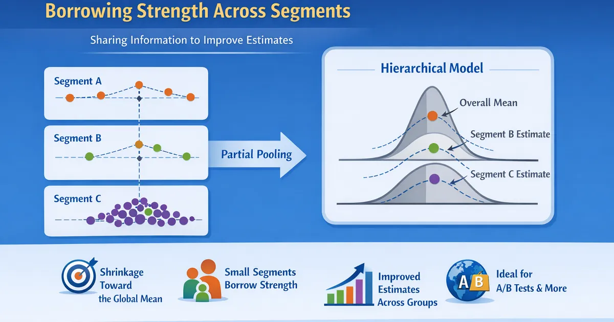
- •Hierarchical models share information across segments -- small segments borrow strength from larger ones
- •Partial pooling is the sweet spot between no pooling (separate estimates) and complete pooling (one estimate for all)
- •Segments with less data are shrunk more toward the global mean; segments with more data keep their own estimate
- •This is ideal for A/B test results by country, user tier, or product category
- •The amount of shrinkage is learned from the data -- you do not have to set it manually
TL;DR
Hierarchical Bayesian models let segments borrow strength from each other. Small segments with noisy data are pulled toward the overall mean, while large segments retain their own estimates. This "partial pooling" gives better estimates than either analyzing each segment separately or ignoring segment differences entirely. This guide covers the intuition, implementation, and practical use cases.
The Problem: Segments with Unequal Data
A Common Scenario
You ran an A/B test globally. Now the PM asks: "What was the effect in each country?"
| Country | Users | Conversions (Control) | Conversions (Treatment) | Observed Lift |
|---|---|---|---|---|
| US | 50,000 | 6,000 | 6,400 | +0.8% |
| UK | 20,000 | 2,400 | 2,560 | +0.8% |
| Germany | 8,000 | 960 | 1,040 | +1.0% |
| Brazil | 2,000 | 240 | 280 | +2.0% |
| Japan | 500 | 55 | 75 | +4.0% |
| Australia | 200 | 22 | 30 | +4.0% |
Japan and Australia show huge lifts, but with tiny sample sizes. Are those real effects or noise?
Three Approaches
- No pooling: Analyze each country separately. Japan's 4% lift has a massive confidence interval. Unreliable.
- Complete pooling: Ignore countries, use the global estimate. Misses real country differences.
- Partial pooling (hierarchical): Share information across countries. Small countries are pulled toward the global mean. Best of both worlds.
How Partial Pooling Works
The Model
Country effect ~ Normal(global_mean, between_country_sd)
Observed data ~ Likelihood(country_effect)
Each country has its own effect, but those effects are drawn from a shared distribution. The model estimates:
- Global mean: The typical effect across all countries
- Between-country SD: How much countries vary
- Country-specific effects: Each country's estimate, shrunk toward the global mean
The Shrinkage Formula
For a simple case, the hierarchical estimate for country j is:
Where the weight depends on the country's sample size relative to the between-country variance:
- Large (lots of data): , keep the country's own estimate
- Small (little data): , shrink toward the global mean
- Large (countries are very different): increases, less shrinkage
Implementation
From Scratch
import numpy as np
from scipy import stats

def hierarchical_model_normal(group_means, group_ses, n_samples=10000):
    """
    Simple hierarchical Normal model via Gibbs sampling.

    group_means: observed mean effect per group
    group_ses: standard error per group
    """
    K = len(group_means)
    y = np.array(group_means)
    se = np.array(group_ses)

    # Initialize
    mu = np.mean(y)  # Global mean
    tau = np.std(y)   # Between-group SD
    theta = y.copy()  # Group effects

    # Storage
    mu_samples = np.zeros(n_samples)
    tau_samples = np.zeros(n_samples)
    theta_samples = np.zeros((n_samples, K))

    for i in range(n_samples):
        # Sample group effects (partial pooling)
        for j in range(K):
            precision = 1/se[j]**2 + 1/tau**2
            post_mean = (y[j]/se[j]**2 + mu/tau**2) / precision
            post_sd = np.sqrt(1/precision)
            theta[j] = np.random.normal(post_mean, post_sd)

        # Sample global mean
        mu_precision = K / tau**2
        mu_post_mean = np.mean(theta)
        mu_post_sd = np.sqrt(tau**2 / K)
        mu = np.random.normal(mu_post_mean, mu_post_sd)

        # Sample between-group SD
        ss = np.sum((theta - mu)**2)
        tau = np.sqrt(ss / np.random.chisquare(K - 1)) if K > 1 else np.abs(np.random.normal(0, 1))

        # Store
        mu_samples[i] = mu
        tau_samples[i] = tau
        theta_samples[i] = theta

    # Discard burn-in
    burn = n_samples // 2
    return {
        'global_mean': mu_samples[burn:],
        'between_sd': tau_samples[burn:],
        'group_effects': theta_samples[burn:],
    }


# Country-level A/B test results
countries = ['US', 'UK', 'Germany', 'Brazil', 'Japan', 'Australia']
observed_lifts = [0.008, 0.008, 0.010, 0.020, 0.040, 0.040]
standard_errors = [0.003, 0.005, 0.008, 0.015, 0.030, 0.050]

result = hierarchical_model_normal(observed_lifts, standard_errors, n_samples=20000)

print("Hierarchical Model Results")
print(f"{'Country':<12} {'Observed':<12} {'Hierarchical':<15} {'Shrinkage'}")
print("-" * 55)
for j, country in enumerate(countries):
    hier_mean = np.mean(result['group_effects'][:, j])
    shrinkage = 1 - (hier_mean - np.mean(observed_lifts)) / (observed_lifts[j] - np.mean(observed_lifts))
    print(f"{country:<12} {observed_lifts[j]:<12.1%} {hier_mean:<15.1%} {shrinkage:.0%}")

global_mean = np.mean(result['global_mean'])
between_sd = np.mean(result['between_sd'])
print(f"\nGlobal mean effect: {global_mean:.1%}")
print(f"Between-country SD: {between_sd:.1%}")
Notice how Japan (4.0% observed) and Australia (4.0% observed) are shrunk substantially toward the global mean, while US and UK (large samples) barely move.
When to Use Hierarchical Models
Classic Product Analytics Use Cases
| Use Case | Groups | What You Estimate |
|---|---|---|
| A/B test by country | Countries | Treatment effect per country |
| Conversion rate by category | Product categories | Category-specific rates |
| Churn by subscription tier | Tiers | Tier-specific churn rates |
| Ad performance by creative | Ad creatives | Click-through rate per creative |
| Feature impact by user segment | User segments | Feature effect per segment |
When Hierarchical Beats Alternatives
def compare_pooling_strategies(true_effects, sample_sizes, noise_sd=0.05,
                                n_simulations=500):
    """
    Compare no pooling, complete pooling, and partial pooling.
    """
    K = len(true_effects)
    mse_no_pool = []
    mse_complete_pool = []
    mse_partial_pool = []

    for _ in range(n_simulations):
        # Simulate observed effects
        observed = [
            true_effects[j] + np.random.normal(0, noise_sd / np.sqrt(sample_sizes[j]))
            for j in range(K)
        ]
        ses = [noise_sd / np.sqrt(n) for n in sample_sizes]

        # No pooling: use observed directly
        mse_no_pool.append(np.mean([(observed[j] - true_effects[j])**2 for j in range(K)]))

        # Complete pooling: use grand mean
        grand_mean = np.mean(observed)
        mse_complete_pool.append(np.mean([(grand_mean - true_effects[j])**2 for j in range(K)]))

        # Partial pooling (simplified shrinkage estimator)
        tau2_hat = max(0, np.var(observed) - np.mean([s**2 for s in ses]))
        weights = [tau2_hat / (tau2_hat + ses[j]**2) if tau2_hat > 0 else 0 for j in range(K)]
        partial = [weights[j]*observed[j] + (1-weights[j])*grand_mean for j in range(K)]
        mse_partial_pool.append(np.mean([(partial[j] - true_effects[j])**2 for j in range(K)]))

    print("Mean Squared Error Comparison")
    print(f"No pooling:       {np.mean(mse_no_pool):.6f}")
    print(f"Complete pooling: {np.mean(mse_complete_pool):.6f}")
    print(f"Partial pooling:  {np.mean(mse_partial_pool):.6f}")
    print(f"\nPartial pooling wins by combining the best of both approaches.")


# Groups with varying sizes
compare_pooling_strategies(
    true_effects=[0.01, 0.012, 0.008, 0.015, 0.009, 0.02],
    sample_sizes=[10000, 5000, 2000, 500, 100, 50]
)
Partial pooling almost always has lower MSE than either extreme.
Practical Considerations
When Not to Use Hierarchical Models
- All groups have large samples: No pooling is fine; shrinkage has negligible effect
- Groups are genuinely unrelated: Borrowing strength from unrelated groups introduces bias
- Only one group: No hierarchy to model (use standard Bayesian regression)
Diagnostics
- Check between-group variance: If tau is near zero, groups are similar and complete pooling is fine. If tau is very large, groups differ so much that no pooling is better.
- Compare shrinkage levels: Groups shrunk more than 50% have estimates heavily influenced by the global mean. This is fine if justified by small sample sizes.
- Posterior predictive checks: Simulate data from the posterior and compare to observed data patterns.
Related Methods
- Bayesian Methods Overview (Pillar) - Full framework
- Bayesian Regression - Shrinkage in regression
- Prior Selection - Priors for hierarchical models
- Practical Bayes Tools - brms makes hierarchical models easy
Key Takeaway
Hierarchical Bayesian models solve the common problem of estimating effects across segments with unequal data. Instead of choosing between noisy individual estimates and a single pooled estimate that ignores segment differences, partial pooling automatically balances both. Small segments borrow strength from the overall pattern while large segments retain their individual signal. Use hierarchical models whenever you analyze experiment results, conversion rates, or user behavior across countries, tiers, categories, or any other grouping.
References
- https://doi.org/10.1017/CBO9780511790942
- https://mc-stan.org/users/documentation/
- https://paul-buerkner.github.io/brms/
Frequently Asked Questions
What is partial pooling?
When should I use a hierarchical model instead of separate models?
How much does a small segment get shrunk?
Key Takeaway
Hierarchical Bayesian models solve the common problem of estimating effects across segments with unequal data. Instead of choosing between noisy individual estimates and a single pooled estimate that ignores segment differences, partial pooling automatically balances both. Small segments borrow strength from the overall pattern while large segments retain their individual signal. Use hierarchical models whenever you analyze experiment results, conversion rates, or user behavior across countries, tiers, categories, or any other grouping.