Contents
Data Transformations: When Log, Sqrt, and Box-Cox Help vs. Mislead
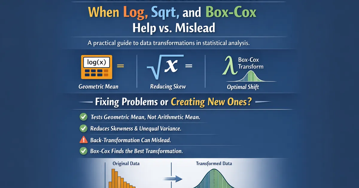
A practical guide to data transformations in statistical analysis. Learn when transformations fix problems, when they create new ones, and how to interpret results correctly.
Quick Hits
- •Log transforms test geometric means, not arithmetic means—know the difference
- •Transformations can fix both skewness and unequal variance simultaneously
- •Back-transformation requires care: mean of logs ≠ log of mean
- •Box-Cox finds the optimal transformation automatically
TL;DR
Transformations can fix assumption violations but change what you're testing. Log transforms test geometric means (appropriate for multiplicative data like revenue, times, ratios); square root helps with counts; Box-Cox finds the optimal power transformation. The critical insight: back-transformed estimates are NOT the same as estimates on the original scale. Know what you're estimating before transforming.
Why Transform Data?
What Transformations Fix
- Skewness: Pull in long tails to symmetrize distribution
- Unequal variance: Often stabilize variance across groups
- Non-linearity: Straighten curved relationships
import numpy as np
from scipy import stats
import matplotlib.pyplot as plt

def demonstrate_transformation_effects():
    """
    Show how transformations affect distribution shape.
    """
    np.random.seed(42)

    # Highly right-skewed data (log-normal)
    original = np.random.lognormal(mean=3, sigma=1, size=500)

    # Transformations
    log_data = np.log(original)
    sqrt_data = np.sqrt(original)

    fig, axes = plt.subplots(1, 3, figsize=(15, 4))

    for ax, data, title in [
        (axes[0], original, f'Original\nSkew: {stats.skew(original):.2f}'),
        (axes[1], log_data, f'Log-transformed\nSkew: {stats.skew(log_data):.2f}'),
        (axes[2], sqrt_data, f'Sqrt-transformed\nSkew: {stats.skew(sqrt_data):.2f}')
    ]:
        ax.hist(data, bins=30, density=True, alpha=0.7)
        ax.set_title(title)
        ax.set_xlabel('Value')

    axes[0].set_ylabel('Density')
    plt.tight_layout()
    return fig


demonstrate_transformation_effects()
Variance Stabilization
def demonstrate_variance_stabilization():
    """
    Show how log transform can equalize group variances.
    """
    np.random.seed(42)

    # Generate data where variance increases with mean
    group_means = [10, 50, 100, 200]
    groups_original = []
    groups_log = []

    for mu in group_means:
        # Variance proportional to mean (common in real data)
        data = np.random.normal(mu, mu * 0.3, 30)
        data = np.maximum(data, 1)  # Keep positive
        groups_original.append(data)
        groups_log.append(np.log(data))

    # Compare variances
    print("Variance Stabilization with Log Transform:")
    print("-" * 50)
    print(f"{'Group Mean':>12} {'Original Var':>15} {'Log Var':>15}")
    print("-" * 50)
    for mu, orig, logged in zip(group_means, groups_original, groups_log):
        print(f"{mu:>12} {np.var(orig, ddof=1):>15.2f} {np.var(logged, ddof=1):>15.4f}")

    # Variance ratio
    orig_ratio = max(np.var(g, ddof=1) for g in groups_original) / \
                 min(np.var(g, ddof=1) for g in groups_original)
    log_ratio = max(np.var(g, ddof=1) for g in groups_log) / \
                min(np.var(g, ddof=1) for g in groups_log)

    print("-" * 50)
    print(f"Variance ratio - Original: {orig_ratio:.1f}, Log: {log_ratio:.1f}")


demonstrate_variance_stabilization()
Log Transformation: The Most Common
When to Use Log Transform
When log transformation is appropriate:
- Right-skewed data (long tail to the right)
- Multiplicative processes (growth rates, ratios, percentages)
- Relative differences matter ("50% more" vs "$50 more")
- Variance proportional to mean (larger values more variable)
- Log-normal distribution (many natural phenomena)
Good candidates: Revenue/income, time durations, concentrations, population sizes, response times, prices
Poor candidates: Differences (can be negative), already symmetric data, data with many zeros, bounded scales (1-5 ratings)
The Critical Insight: What Are You Testing?
def geometric_vs_arithmetic_mean():
    """
    Demonstrate the difference between arithmetic and geometric means.
    """
    np.random.seed(42)

    # Two groups with log-normal data
    group1 = np.random.lognormal(mean=4, sigma=0.5, size=100)
    group2 = np.random.lognormal(mean=4.2, sigma=0.5, size=100)  # 20% higher geometric mean

    # Arithmetic means
    arith_mean1 = np.mean(group1)
    arith_mean2 = np.mean(group2)
    arith_diff = arith_mean2 - arith_mean1
    arith_ratio = arith_mean2 / arith_mean1

    # Geometric means (exp of mean of logs)
    geom_mean1 = np.exp(np.mean(np.log(group1)))
    geom_mean2 = np.exp(np.mean(np.log(group2)))
    geom_diff = geom_mean2 - geom_mean1
    geom_ratio = geom_mean2 / geom_mean1

    print("Arithmetic vs. Geometric Means")
    print("=" * 50)
    print(f"\n{'':20} {'Group 1':>12} {'Group 2':>12}")
    print("-" * 50)
    print(f"{'Arithmetic Mean':20} {arith_mean1:>12.2f} {arith_mean2:>12.2f}")
    print(f"{'Geometric Mean':20} {geom_mean1:>12.2f} {geom_mean2:>12.2f}")
    print()
    print("Comparisons:")
    print("-" * 50)
    print(f"Arithmetic: Group 2 is ${arith_diff:.2f} more (ratio: {arith_ratio:.2f})")
    print(f"Geometric: Group 2 is ${geom_diff:.2f} more (ratio: {geom_ratio:.2f})")
    print()
    print("Key insight: Log transform tests the RATIO (geometric mean)")
    print("If you want to test 'how much more money', use original scale")
    print("If you want to test 'what multiplier', use log scale")


geometric_vs_arithmetic_mean()
Proper Back-Transformation
def proper_back_transformation():
    """
    Show correct back-transformation for log data.
    """
    np.random.seed(42)

    # Treatment increases geometric mean by 20%
    control = np.random.lognormal(mean=4, sigma=0.5, size=100)
    treatment = np.random.lognormal(mean=4 + np.log(1.2), sigma=0.5, size=100)

    # Analysis on log scale
    log_control = np.log(control)
    log_treatment = np.log(treatment)

    diff_log = np.mean(log_treatment) - np.mean(log_control)
    se_diff = np.sqrt(np.var(log_control, ddof=1)/100 +
                      np.var(log_treatment, ddof=1)/100)

    # Confidence interval on log scale
    ci_low_log = diff_log - 1.96 * se_diff
    ci_high_log = diff_log + 1.96 * se_diff

    print("Back-Transformation of Log Results")
    print("=" * 50)
    print()
    print("On log scale:")
    print(f"  Difference: {diff_log:.4f}")
    print(f"  95% CI: [{ci_low_log:.4f}, {ci_high_log:.4f}]")
    print()
    print("Back-transformed (CORRECT):")
    print(f"  Ratio: {np.exp(diff_log):.3f} (treatment/control)")
    print(f"  95% CI for ratio: [{np.exp(ci_low_log):.3f}, {np.exp(ci_high_log):.3f}]")
    print()
    print("Interpretation: Treatment is {:.1%} higher".format(np.exp(diff_log) - 1))
    print()
    print("WRONG interpretation would be:")
    print(f"  exp(mean_treatment) - exp(mean_control) = {np.exp(np.mean(log_treatment)) - np.exp(np.mean(log_control)):.2f}")
    print("  (This is NOT the same as the difference in arithmetic means)")


proper_back_transformation()
Handling Zeros
The Problem
def demonstrate_zero_problem():
    """
    Show why zeros are problematic for log transforms.
    """
    # Data with zeros (common in revenue, engagement, etc.)
    data = [0, 0, 0, 5, 10, 15, 20, 50, 100, 500]

    print("The Zero Problem:")
    print("-" * 40)
    print(f"Data: {data}")
    print(f"log(0) = undefined (negative infinity)")
    print()
    print("Common 'solutions' and their issues:")
    print()
    print("1. Add small constant: log(x + 1)")
    print(f"   Result: {[np.log(x + 1) for x in data]}")
    print("   Issue: Arbitrary choice, affects results")
    print()
    print("2. Add small epsilon: log(x + 0.001)")
    print(f"   Result: {[f'{np.log(x + 0.001):.2f}' for x in data]}")
    print("   Issue: Very different from log(x + 1)")
    print()
    print("3. Replace zeros with minimum positive value")
    min_positive = min(x for x in data if x > 0)
    print(f"   Minimum positive: {min_positive}")
    print("   Issue: Still arbitrary")


demonstrate_zero_problem()
Better Approaches
| Approach | Description | When to use | Example |
|---|---|---|---|
| Two-part model | Separate model for P(zero) and E[Y|Y>0] | Zeros have different meaning than small values | Revenue (non-purchasers vs purchasers) |
| Rank-based methods | Use Mann-Whitney, Kruskal-Wallis | Don't need parametric assumptions | General comparison with heavy zeros |
| Inverse hyperbolic sine | asinh(x) ≈ log(2x) for large x, handles 0 | Want log-like transform that handles zeros | Economic data with true zeros |
| Poisson/negative binomial | Count models that naturally handle zeros | Count data | Number of purchases, sessions, etc. |
def inverse_hyperbolic_sine_demo():
    """
    Demonstrate IHS transform as zero-friendly alternative.
    """
    x = np.array([0, 1, 5, 10, 50, 100, 500, 1000])

    print("Inverse Hyperbolic Sine vs. Log Transform:")
    print("-" * 60)
    print(f"{'x':>8} {'log(x)':>12} {'log(x+1)':>12} {'asinh(x)':>12}")
    print("-" * 60)
    for val in x:
        log_x = 'undefined' if val == 0 else f'{np.log(val):.3f}'
        log_x1 = f'{np.log(val + 1):.3f}'
        asinh_x = f'{np.arcsinh(val):.3f}'
        print(f"{val:>8} {log_x:>12} {log_x1:>12} {asinh_x:>12}")

    print("\nNote: asinh(x) ≈ log(2x) for large x")


inverse_hyperbolic_sine_demo()
Square Root Transformation
When to Use
When square root transformation is appropriate:
- Count data (Poisson-distributed counts)
- Moderate skew (less aggressive than log)
- Variance proportional to mean (but not as severely as log-normal)
Good for: Count of events (clicks, purchases), species counts in ecology, defect counts in quality control
Sqrt is gentler than log — use when log over-corrects.
def compare_sqrt_and_log():
    """
    Compare sqrt and log transforms.
    """
    np.random.seed(42)

    # Poisson data (counts)
    counts = np.random.poisson(lam=10, size=200)

    # Skewness under different transforms
    skew_original = stats.skew(counts)
    skew_sqrt = stats.skew(np.sqrt(counts))
    skew_log = stats.skew(np.log(counts + 1))

    print("Comparing Transforms for Count Data:")
    print("-" * 40)
    print(f"Original skewness: {skew_original:.3f}")
    print(f"Sqrt skewness: {skew_sqrt:.3f}")
    print(f"Log(x+1) skewness: {skew_log:.3f}")
    print()
    print("For Poisson counts, sqrt often works well.")
    print("Log may over-correct, making data left-skewed.")


compare_sqrt_and_log()
Box-Cox Transformation
Automatic Power Selection
The Box-Cox transformation finds the optimal power λ:
from scipy.stats import boxcox, boxcox_normmax

def boxcox_demonstration():
    """
    Demonstrate Box-Cox transformation.
    """
    np.random.seed(42)

    # Highly skewed positive data
    data = np.random.lognormal(mean=3, sigma=1.5, size=200)

    # Find optimal lambda
    data_transformed, lambda_opt = boxcox(data)

    # Common lambda interpretations
    interpretations = {
        -1: 'Reciprocal (1/y)',
        -0.5: 'Reciprocal square root',
        0: 'Log',
        0.5: 'Square root',
        1: 'No transformation',
        2: 'Square'
    }

    print("Box-Cox Transformation")
    print("=" * 50)
    print(f"\nOptimal λ: {lambda_opt:.3f}")
    print()
    print("Common λ values and their transforms:")
    for lam, interp in interpretations.items():
        print(f"  λ = {lam:>4}: {interp}")

    print(f"\nSkewness before: {stats.skew(data):.3f}")
    print(f"Skewness after: {stats.skew(data_transformed):.3f}")

    # Closest interpretation
    closest = min(interpretations.keys(), key=lambda x: abs(x - lambda_opt))
    print(f"\nNearest standard transform: {interpretations[closest]}")


boxcox_demonstration()


def boxcox_practical_workflow(data, alpha=0.05):
    """
    Practical Box-Cox workflow with confidence interval for lambda.
    """
    # Ensure positive
    if np.any(data <= 0):
        raise ValueError("Box-Cox requires strictly positive data")

    # Find optimal lambda
    data_transformed, lambda_opt = boxcox(data)

    # Get confidence interval for lambda
    # Use profile likelihood
    from scipy.optimize import minimize_scalar

    n = len(data)
    log_data = np.log(data)
    sum_log = np.sum(log_data)

    def neg_log_likelihood(lam):
        if abs(lam) < 1e-10:
            y = log_data
        else:
            y = (data**lam - 1) / lam
        return n/2 * np.log(np.var(y, ddof=0)) - (lam - 1) * sum_log

    # Calculate confidence interval (simplified)
    ll_opt = neg_log_likelihood(lambda_opt)
    threshold = ll_opt + stats.chi2.ppf(1 - alpha, 1) / 2

    # Search for CI bounds
    ci_low = lambda_opt - 1
    ci_high = lambda_opt + 1

    for lam in np.linspace(lambda_opt - 2, lambda_opt, 100):
        if neg_log_likelihood(lam) <= threshold:
            ci_low = lam
            break

    for lam in np.linspace(lambda_opt + 2, lambda_opt, 100):
        if neg_log_likelihood(lam) <= threshold:
            ci_high = lam
            break

    return {
        'lambda_opt': lambda_opt,
        'lambda_ci': (ci_low, ci_high),
        'transformed_data': data_transformed,
        'recommendation': get_lambda_recommendation(lambda_opt, ci_low, ci_high)
    }


def get_lambda_recommendation(lambda_opt, ci_low, ci_high):
    """
    Recommend a standard transformation based on Box-Cox.
    """
    standard_lambdas = [-1, -0.5, 0, 0.5, 1]
    names = ['reciprocal', 'reciprocal sqrt', 'log', 'sqrt', 'none']

    for lam, name in zip(standard_lambdas, names):
        if ci_low <= lam <= ci_high:
            return f"Use {name} (λ={lam} in CI)"

    return f"Use optimal λ={lambda_opt:.2f} (no standard transform in CI)"
Common Mistakes
Mistake 1: Transforming When Not Needed
def transformation_necessity_check(data, groups=None):
    """
    Check if transformation is actually necessary.
    """
    n = len(data)
    skew = stats.skew(data)

    print("Do You Need to Transform?")
    print("-" * 40)
    print(f"Sample size: {n}")
    print(f"Skewness: {skew:.3f}")

    if n >= 50 and abs(skew) < 1:
        print("\n✓ Probably NOT needed:")
        print("  - Large sample size")
        print("  - Moderate skewness")
        print("  - CLT will help")
    elif n >= 30 and abs(skew) < 0.5:
        print("\n✓ Probably NOT needed:")
        print("  - Adequate sample size")
        print("  - Mild skewness")
    elif abs(skew) > 2:
        print("\n⚠️  Consider transformation:")
        print("  - Substantial skewness")
        print("  - May affect inference")
    else:
        print("\nBorderline - transformation optional")
        print("Consider robust methods as alternative")
Mistake 2: Wrong Back-Transformation
def back_transformation_mistakes():
    """
    Common back-transformation errors.
    """
    np.random.seed(42)
    data = np.random.lognormal(3, 1, 100)

    log_mean = np.mean(np.log(data))
    log_se = np.std(np.log(data), ddof=1) / np.sqrt(100)

    print("Back-Transformation Errors")
    print("=" * 50)
    print()
    print("CORRECT:")
    print(f"  Geometric mean = exp(mean of logs) = {np.exp(log_mean):.2f}")
    print(f"  95% CI for geom mean: [{np.exp(log_mean - 1.96*log_se):.2f}, "
          f"{np.exp(log_mean + 1.96*log_se):.2f}]")
    print()
    print("COMMON MISTAKES:")
    print(f"  ✗ exp(mean(log(x))) ≠ mean(x)")
    print(f"    Geometric mean: {np.exp(log_mean):.2f}")
    print(f"    Arithmetic mean: {np.mean(data):.2f}")
    print()
    print(f"  ✗ exp(CI for log mean) is CI for GEOMETRIC mean,")
    print(f"    not arithmetic mean")


back_transformation_mistakes()
Mistake 3: Transforming Outcome in Regression
When you fit log(y) ~ x, you're estimating , not . These are not the same.
By Jensen's inequality:
Predictions from log-linear models need correction (Duan's smearing estimator or similar).
Transformation Decision Guide
def transformation_decision_tree(data, has_zeros=False):
    """
    Guide for choosing transformation.
    """
    skew = stats.skew(data)
    n = len(data)

    print("TRANSFORMATION DECISION GUIDE")
    print("=" * 50)
    print(f"\nData characteristics:")
    print(f"  n = {n}")
    print(f"  Skewness = {skew:.2f}")
    print(f"  Has zeros = {has_zeros}")
    print(f"  Min value = {np.min(data):.2f}")

    print("\nDecision:")
    print("-" * 40)

    if abs(skew) < 0.5:
        print("Minimal skew → No transformation needed")
    elif has_zeros:
        print("Data has zeros:")
        print("  - Consider two-part model")
        print("  - Or rank-based methods")
        print("  - Or asinh transform")
        print("  - Avoid log(x + constant)")
    elif skew > 2:
        print("Strong right skew:")
        print("  - Log transform likely appropriate")
        print("  - Verify multiplicative structure")
        print("  - Remember: testing geometric means")
    elif skew > 1:
        print("Moderate right skew:")
        print("  - Try sqrt first (less aggressive)")
        print("  - Log if sqrt insufficient")
        print("  - Or use robust methods without transform")
    elif skew < -1:
        print("Left skew (unusual):")
        print("  - Square transform may help")
        print("  - Or reflect data: max(x) - x")
    else:
        print("Mild skew → Consider:")
        print("  - No transformation (CLT if n > 30)")
        print("  - Robust methods")
        print("  - Box-Cox for optimization")


# Example
np.random.seed(42)
revenue_data = np.random.lognormal(4, 1.5, 100)
transformation_decision_tree(revenue_data, has_zeros=False)
R Implementation
# Transformation workflow in R

transformation_analysis <- function(data) {
  library(MASS)  # for boxcox

  cat("TRANSFORMATION ANALYSIS\n")
  cat(rep("=", 50), "\n\n")

  # Original statistics
  cat("Original data:\n")
  cat(sprintf("  n: %d\n", length(data)))
  cat(sprintf("  Mean: %.2f\n", mean(data)))
  cat(sprintf("  Skewness: %.3f\n", e1071::skewness(data)))

  # Try different transforms
  transforms <- list(
    original = data,
    log = log(data),
    sqrt = sqrt(data)
  )

  cat("\nSkewness by transform:\n")
  for (name in names(transforms)) {
    cat(sprintf("  %s: %.3f\n", name, e1071::skewness(transforms[[name]])))
  }

  # Box-Cox (requires positive data)
  if (all(data > 0)) {
    # Fit simple model for Box-Cox
    bc <- boxcox(data ~ 1, plotit = FALSE)
    lambda_opt <- bc$x[which.max(bc$y)]
    cat(sprintf("\nBox-Cox optimal λ: %.3f\n", lambda_opt))
  }

  # Visual comparison
  par(mfrow = c(1, 3))
  hist(data, main = "Original", probability = TRUE)
  if (all(data > 0)) hist(log(data), main = "Log", probability = TRUE)
  hist(sqrt(data), main = "Sqrt", probability = TRUE)
  par(mfrow = c(1, 1))
}

# Usage:
# data <- rlnorm(200, meanlog = 3, sdlog = 1)
# transformation_analysis(data)
Related Methods
- Assumption Checks Master Guide — The pillar article
- Why Revenue Is Hard — Revenue-specific challenges
- Robust Statistics Toolbox — Alternatives to transformation
- Dealing with Zeros — Zero-inflated data
Key Takeaway
Transformations are powerful but change what you're estimating. Log transforms test geometric means (ratios), not arithmetic means (differences). Before transforming, ask: Does my research question concern relative or absolute differences? If absolute, keep the original scale and use robust methods. If relative, log is appropriate. Always report results on the interpretable scale with correct back-transformation.
References
- https://www.jstor.org/stable/2683401
- https://doi.org/10.1080/00031305.1990.10475748
- Bland, J. M., & Altman, D. G. (1996). The use of transformation when comparing two means. *BMJ*, 312(7039), 1153.
- Feng, C., Wang, H., Lu, N., Chen, T., He, H., Lu, Y., & Tu, X. M. (2014). Log-transformation and its implications for data analysis. *Shanghai Archives of Psychiatry*, 26(2), 105.
- Box, G. E., & Cox, D. R. (1964). An analysis of transformations. *Journal of the Royal Statistical Society: Series B*, 26(2), 211-243.
Frequently Asked Questions
When should I log-transform my data?
How do I handle zeros with log transform?
Should I report results on the transformed or original scale?
Key Takeaway
Data transformations are powerful tools for meeting assumptions, but they change what you're estimating. Log transforms shift the question from 'how much bigger?' to 'how many times bigger?' This may or may not match your research question. Always understand what the transformation does to your estimand before applying it.