Contents
Why Revenue Is Hard: Log-Normal Distributions and Heavy Tails
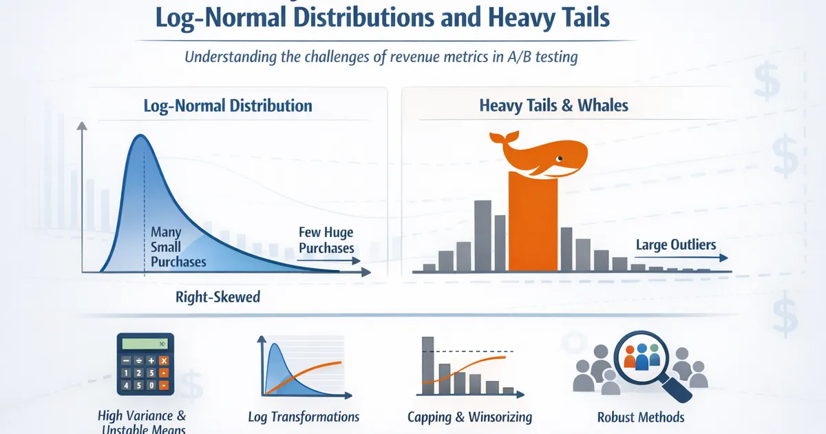
A deep dive into why revenue metrics are statistically challenging. Learn about log-normal distributions, heavy tails, whale effects, and practical approaches to analyzing revenue in A/B tests.
Quick Hits
- •Revenue is typically right-skewed: many small values, few very large ones
- •A single whale can shift your experiment's mean by more than the treatment effect
- •Standard errors on revenue metrics are huge - you need massive samples
- •Log transformation helps but changes the question (geometric vs. arithmetic mean)
- •Capping/Winsorizing is common but requires disclosure and sensitivity analysis
TL;DR
Revenue data is statistically difficult because it combines three challenges: many zeros (non-purchasers), right-skew (most purchases are small), and heavy tails (occasional large purchases). A single "whale" customer can shift your experiment's mean by more than your treatment effect. Standard t-tests have poor power and unstable results. Solutions include log transformation (changes interpretation), capping/Winsorization (reduces extreme influence), and CUPED (reduces variance).
The Three Challenges of Revenue
Challenge 1: Many Zeros
In most products, the majority of users don't purchase:
- E-commerce: 2-5% conversion rate → 95-98% zeros
- SaaS with free tier: 5-15% paid → 85-95% zeros
- Games: 1-5% paying players → 95-99% zeros
Problem: Can't log-transform zeros. Two distinct populations (purchasers vs. non-purchasers).
Challenge 2: Right Skew
Among purchasers, most buy small amounts:
- Many $10-50 purchases
- Some $100-500 purchases
- Few $1000+ purchases
Problem: Mean is much higher than median. "Average" doesn't represent typical behavior.
Challenge 3: Heavy Tails
The top 1% of customers often generate 50%+ of revenue:
- Whales: Individual customers spending the median
- Not outliers—they're part of your business model
Problem: A few extreme values dominate sample statistics.
The Whale Problem
One Customer, Big Impact
Example:
- Control: 10,000 users, mean revenue = $5.00
- Treatment: 10,000 users, mean revenue = $5.30
Looks like a 6% lift! But...
One treatment user spent $3,500 (a whale). Remove that whale: Treatment mean = $4.95
The whale contributed half the observed effect.
Why This Matters
| Scenario | Conclusion |
|---|---|
| Whale in treatment | False positive (inflated effect) |
| Whale in control | False negative (hidden real effect) |
| Random | High variance, low power |
Whale assignment is random, but their impact is huge.
Math: Why Heavy Tails = Huge Variance
For a log-normal distribution with mean and variance on the log scale:
Variance grows exponentially with . With typical revenue parameters, variance can be the squared mean.
What "Heavy Tails" Actually Means
Tail Behavior
Normal distribution: 99.7% of values within 3 standard deviations
Heavy-tailed: Extreme values occur much more often than normal predicts
Example:
| Metric | Normal (SD=10) | Log-Normal () |
|---|---|---|
| P(X > 30) | 0.1% | 5% |
| P(X > 50) | ~0% | 1% |
| P(X > 100) | ~0% | 0.1% |
Impact on Statistics
| Property | Normal | Heavy-Tailed |
|---|---|---|
| CLT convergence | Fast (~30 samples) | Slow (100s-1000s) |
| Mean stability | Good | Poor |
| Outlier influence | Limited | Dominant |
| Required sample size | Moderate | Large |
Code: Simulating the Problem
import numpy as np
import pandas as pd
from scipy import stats
import matplotlib.pyplot as plt


def simulate_revenue_experiment(n_per_group=5000, true_lift=0.05, n_simulations=1000):
    """
    Simulate revenue A/B tests to show the whale problem.
    """
    results = []

    for sim in range(n_simulations):
        # Generate control revenue
        # 70% zeros, 30% log-normal purchases
        is_purchaser_c = np.random.binomial(1, 0.3, n_per_group)
        revenue_c = np.where(
            is_purchaser_c,
            np.random.lognormal(mean=2.5, sigma=1.5, size=n_per_group),
            0
        )

        # Treatment: slightly higher mean log revenue
        is_purchaser_t = np.random.binomial(1, 0.3, n_per_group)
        revenue_t = np.where(
            is_purchaser_t,
            np.random.lognormal(mean=2.5 + np.log(1 + true_lift), sigma=1.5, size=n_per_group),
            0
        )

        # Standard t-test
        t_stat, p_value = stats.ttest_ind(revenue_c, revenue_t)

        # Effect estimate
        mean_c = np.mean(revenue_c)
        mean_t = np.mean(revenue_t)
        observed_lift = (mean_t - mean_c) / mean_c if mean_c > 0 else 0

        # Check for whale influence
        max_c = np.max(revenue_c)
        max_t = np.max(revenue_t)
        whale_influence = max(max_c, max_t) / (n_per_group * max(mean_c, mean_t))

        results.append({
            'mean_control': mean_c,
            'mean_treatment': mean_t,
            'observed_lift': observed_lift,
            'p_value': p_value,
            'significant': p_value < 0.05,
            'max_control': max_c,
            'max_treatment': max_t,
            'whale_influence': whale_influence
        })

    return pd.DataFrame(results)


def analyze_simulation_results(results, true_lift):
    """
    Analyze simulation results.
    """
    print("Revenue A/B Test Simulation Results")
    print("=" * 50)
    print(f"True lift: {true_lift:.1%}")
    print(f"\nObserved lift distribution:")
    print(f"  Mean: {results['observed_lift'].mean():.1%}")
    print(f"  Median: {results['observed_lift'].median():.1%}")
    print(f"  Std Dev: {results['observed_lift'].std():.1%}")
    print(f"  Min: {results['observed_lift'].min():.1%}")
    print(f"  Max: {results['observed_lift'].max():.1%}")

    print(f"\nPower (correctly detect true effect):")
    print(f"  Significant and lift > 0: {(results['significant'] & (results['observed_lift'] > 0)).mean():.1%}")

    print(f"\nEffect of whales:")
    high_whale = results['whale_influence'] > results['whale_influence'].median()
    print(f"  High whale experiments - Lift std: {results.loc[high_whale, 'observed_lift'].std():.1%}")
    print(f"  Low whale experiments - Lift std: {results.loc[~high_whale, 'observed_lift'].std():.1%}")


# Run simulation
np.random.seed(42)
results = simulate_revenue_experiment(n_per_group=5000, true_lift=0.05, n_simulations=1000)
analyze_simulation_results(results, 0.05)

# Plot distribution of observed effects
fig, axes = plt.subplots(1, 2, figsize=(12, 4))

axes[0].hist(results['observed_lift'], bins=50, edgecolor='white')
axes[0].axvline(0.05, color='red', linestyle='--', label='True lift')
axes[0].axvline(results['observed_lift'].mean(), color='blue', linestyle='--', label='Mean observed')
axes[0].set_xlabel('Observed Lift')
axes[0].set_ylabel('Count')
axes[0].set_title('Distribution of Observed Lift')
axes[0].legend()

axes[1].scatter(results['max_treatment'], results['observed_lift'], alpha=0.3)
axes[1].axhline(0.05, color='red', linestyle='--')
axes[1].set_xlabel('Max Treatment Revenue (Whale Size)')
axes[1].set_ylabel('Observed Lift')
axes[1].set_title('Whale Impact on Observed Lift')

plt.tight_layout()
plt.show()
Solutions
Solution 1: Log Transformation
Transform to log scale, where data is more normal.
# Log-transform non-zero values
revenue_log = np.log(revenue[revenue > 0])

# Run t-test on log values
t_stat, p_value = stats.ttest_ind(log_control, log_treatment)

# Effect is ratio (geometric mean)
log_diff = np.mean(log_treatment) - np.mean(log_control)
ratio = np.exp(log_diff)  # e.g., 1.05 = 5% higher geometric mean
Pros: Well-behaved statistics Cons: Ignores zeros, measures geometric mean (not total revenue)
Solution 2: Winsorization/Capping
Cap extreme values at a percentile.
def winsorize(x, lower=0.01, upper=0.99):
    """Cap values at percentiles."""
    lower_bound = np.percentile(x, lower * 100)
    upper_bound = np.percentile(x, upper * 100)
    return np.clip(x, lower_bound, upper_bound)

revenue_capped = winsorize(revenue, lower=0, upper=0.99)
Pros: Reduces whale influence, keeps all users Cons: Somewhat arbitrary cutoff, requires disclosure
Solution 3: CUPED (Variance Reduction)
Use pre-experiment data to reduce variance.
# Pre-experiment revenue
pre_revenue = data['pre_experiment_revenue']
post_revenue = data['experiment_revenue']

# CUPED adjustment
theta = np.cov(post_revenue, pre_revenue)[0, 1] / np.var(pre_revenue)
adjusted_revenue = post_revenue - theta * (pre_revenue - np.mean(pre_revenue))
Pros: Can reduce variance 20-50%, preserves mean interpretation Cons: Requires pre-experiment data
Solution 4: Trimmed Means
Remove top/bottom X% before computing mean.
from scipy.stats import trim_mean

# 5% trimmed mean (removes top and bottom 5%)
trimmed_control = trim_mean(revenue_control, 0.05)
trimmed_treatment = trim_mean(revenue_treatment, 0.05)
Pros: Robust to extremes Cons: Changes what you're measuring
Solution 5: Quantile Analysis
Report effects at different percentiles.
for pct in [50, 75, 90, 95]:
    q_c = np.percentile(revenue_control, pct)
    q_t = np.percentile(revenue_treatment, pct)
    print(f"P{pct}: Control={q_c:.2f}, Treatment={q_t:.2f}")
Pros: Rich picture of distribution shift Cons: More complex to interpret
Comparison of Methods
| Method | Handles Zeros | Robust to Whales | Estimates Total Revenue | Interpretable |
|---|---|---|---|---|
| Standard t-test | Yes | No | Yes | Yes |
| Log transformation | No | Yes | No (geometric mean) | Moderate |
| Winsorization | Yes | Yes | Approx | Yes |
| CUPED | Yes | Partial | Yes | Yes |
| Trimmed mean | Yes | Yes | No (subset) | Moderate |
| Bootstrap | Yes | Partial | Yes | Yes |
Reporting Guidelines
When Using Modified Methods
Always disclose:
- What modification you used (capping at 99th percentile, 10% trim, etc.)
- Why (high variance due to heavy tails)
- Sensitivity analysis (results with and without modification)
Example:
"Revenue was capped at the 99th percentile ($500) to reduce whale-driven variance. With capping: +5.2% lift (95% CI: 2.1% to 8.3%, ) Without capping: +4.8% lift (95% CI: -3.2% to 12.8%, )"
Sample Size Implications
Expect to need the sample size for revenue vs. conversion rates.
| Metric | Typical MDE | Typical n per group |
|---|---|---|
| Conversion rate | 5% relative | 10,000-50,000 |
| Revenue per user | 5% relative | 50,000-500,000 |
Related Methods
- Metric Distributions (Pillar) - Full distributions overview
- Winsorization and Trimming - Outlier handling details
- Bootstrap for Heavy-Tailed Metrics - Non-parametric approach
- CUPED and Variance Reduction - Pre-experiment adjustment
Key Takeaway
Revenue metrics are challenging because they combine zeros, right-skew, and heavy tails. A single whale customer can dominate your experiment. Standard t-tests are technically valid but have poor power and unstable estimates. Use a combination of approaches: variance reduction (CUPED), outlier handling (Winsorization), and sensitivity analysis. Always report what you did and why—transparency about methodology is essential when analyzing heavy-tailed metrics.
References
- https://www.kdd.org/kdd2016/papers/files/Paper_573.pdf
- https://arxiv.org/abs/1803.06336
- https://engineering.linkedin.com/blog/2019/variance-reduction
- Deng, A., & Shi, X. (2016). Data-driven metric development for online controlled experiments: Seven lessons learned. *KDD*, 77-86.
- Wager, S., & Athey, S. (2018). Estimation and inference of heterogeneous treatment effects using random forests. *JASA*, 113(523), 1228-1242.
- Poyarkov, A., et al. (2016). Boosted decision tree regression adjustment for variance reduction in online controlled experiments. *KDD*, 235-244.
Frequently Asked Questions
Why can't I just use a t-test on revenue?
Should I exclude whales from my analysis?
How do I know if my data is log-normal?
Key Takeaway
Revenue metrics combine three challenges: zeros (non-purchasers), right-skew (most purchases are small), and heavy tails (occasional very large purchases). This makes means unstable, standard errors huge, and power low. Address with transformation, capping, robust methods, or specialized models—but always understand how your choice affects interpretation.