Contents
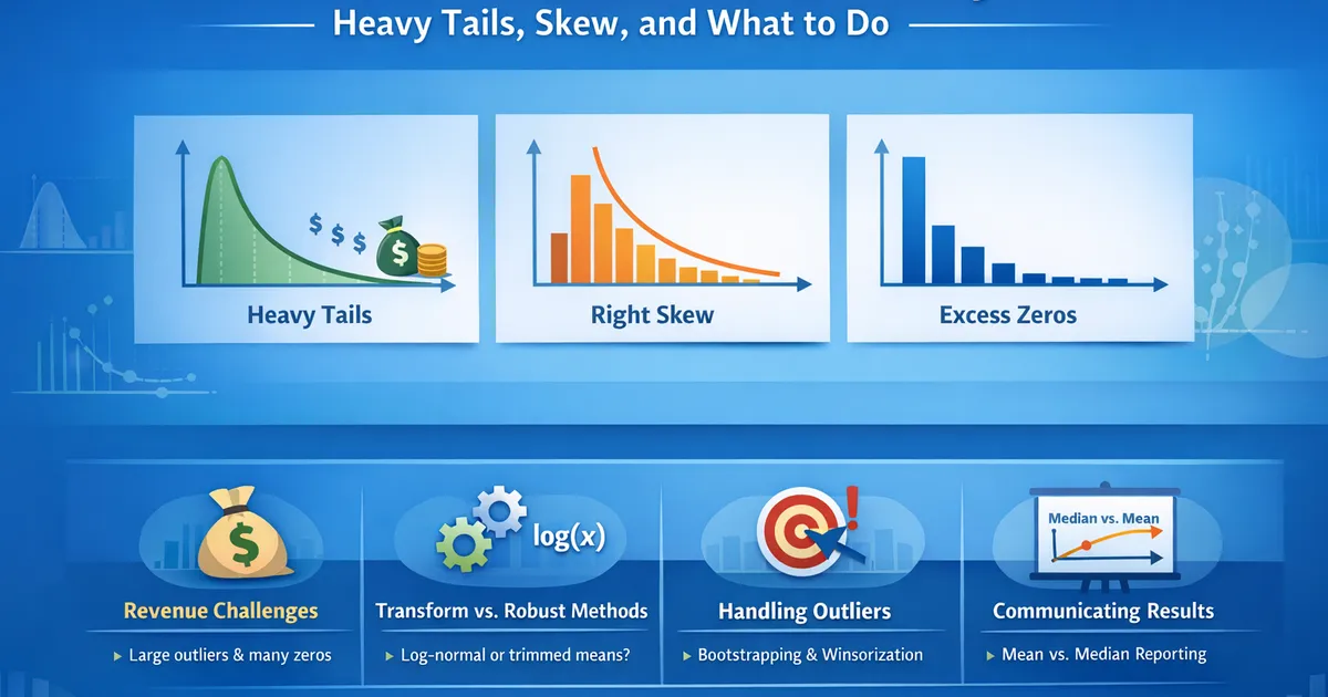
Metric Distributions in Product Analytics: Heavy Tails, Skew, and What to Do
A comprehensive guide to handling real-world metric distributions in product analytics. Learn why revenue is hard, how to deal with zeros, when to transform vs. use robust methods, and how to communicate results on skewed data.
Quick Hits
- •Most product metrics are NOT normal - revenue, engagement, time are typically right-skewed
- •Heavy tails mean extreme values dominate the mean and inflate variance
- •Standard t-tests can fail badly on revenue data - consider trimmed means or bootstrap
- •Zeros complicate everything - can't log-transform, may need two-part models
- •Choose your summary statistic carefully: mean, median, and trimmed mean answer different questions
TL;DR
Most product metrics don't follow normal distributions. Revenue is right-skewed with heavy tails, engagement metrics have excess zeros, and latency has long tails. This matters because standard statistical methods assume normality and can give wrong answers on skewed data. This guide covers why certain metrics are problematic, how to diagnose distributional issues, and practical approaches—transformation, robust methods, and specialized models—for each situation.
Why Distributions Matter
The Normal Assumption
Standard methods (t-tests, ANOVA, regression) assume:
- Data is approximately normal, OR
- Enough data that the Central Limit Theorem kicks in
When This Fails
Heavy tails and skew cause:
- Unstable means: A few extreme values dominate
- Inflated variance: Standard errors are large and unstable
- Poor CI coverage: 95% CIs may cover the true mean only 80% of the time
- Underpowered tests: Variance is so high you can't detect real effects
The CLT Doesn't Always Save You
The Central Limit Theorem says the sampling distribution of the mean approaches normal with large n. But for heavy-tailed distributions:
- "Large n" can mean thousands, not hundreds
- Extreme values can occur in your sample with reasonable probability
- One whale can dominate your entire experiment
Common Problematic Distributions
1. Revenue and Monetary Metrics
Characteristics:
- Many zeros (non-payers)
- Right-skewed (most purchases are small)
- Heavy tail (occasional large purchases)
- Often log-normal among purchasers
Why it's hard: The mean is dominated by rare large values, variance is enormous, and zeros prevent simple log transformation.
2. Engagement Counts
Characteristics:
- Zero-inflated (many inactive users)
- Right-skewed (power users dominate)
- Discrete (can't have 2.5 sessions)
Why it's hard: Two populations (inactive and active) mixed together, standard Poisson doesn't fit.
3. Time and Latency
Characteristics:
- Strictly positive
- Right-skewed
- Long tail (occasional very slow responses)
Why it's hard: A few slow requests inflate the mean, percentiles (p50, p95) are more meaningful than mean.
4. Conversion and Binary Metrics
Characteristics:
- Bernoulli (0 or 1)
- Often low rates (1-10%)
Why it's hard: Variance depends on mean, very low rates need large samples, normal approximation can fail.
Diagnosing Your Distribution
Quick Checks
| Check | What It Tells You |
|---|---|
| Mean vs. Median | If mean >> median, right-skewed |
| SD vs. Mean | If SD > mean, likely heavy-tailed |
| Min, Max | Extreme values relative to median |
| Histogram shape | Visual check for skew, modes, zeros |
Code: Distribution Diagnostics
import numpy as np
import pandas as pd
import matplotlib.pyplot as plt
from scipy import stats


def diagnose_distribution(data, name='metric'):
    """
    Comprehensive distribution diagnostics for product metrics.
    """
    # Remove NaN
    x = data.dropna().values

    # Basic statistics
    n = len(x)
    mean = np.mean(x)
    median = np.median(x)
    std = np.std(x)
    skew = stats.skew(x)
    kurtosis = stats.kurtosis(x)  # Excess kurtosis (0 = normal)

    # Zero proportion
    zero_pct = (x == 0).sum() / n

    # Percentiles
    pcts = np.percentile(x, [5, 25, 50, 75, 95, 99])

    # Flags
    flags = []
    if mean > 2 * median and median > 0:
        flags.append("⚠️ Heavy right skew (mean >> median)")
    if std > mean and mean > 0:
        flags.append("⚠️ High variance (SD > mean)")
    if zero_pct > 0.2:
        flags.append(f"⚠️ Many zeros ({zero_pct:.0%})")
    if kurtosis > 3:
        flags.append(f"⚠️ Heavy tails (kurtosis = {kurtosis:.1f})")
    if skew > 2:
        flags.append(f"⚠️ Strong skew ({skew:.1f})")

    # Report
    report = {
        'name': name,
        'n': n,
        'mean': mean,
        'median': median,
        'std': std,
        'skewness': skew,
        'kurtosis': kurtosis,
        'zero_pct': zero_pct,
        'percentiles': dict(zip(['p5', 'p25', 'p50', 'p75', 'p95', 'p99'], pcts)),
        'flags': flags
    }

    return report


def plot_distribution(data, name='metric', figsize=(14, 4)):
    """
    Visualize distribution with histogram and Q-Q plot.
    """
    x = data.dropna().values

    fig, axes = plt.subplots(1, 3, figsize=figsize)

    # Histogram
    ax1 = axes[0]
    ax1.hist(x, bins=50, edgecolor='white', alpha=0.7)
    ax1.axvline(np.mean(x), color='red', linestyle='--', label=f'Mean={np.mean(x):.2f}')
    ax1.axvline(np.median(x), color='blue', linestyle='--', label=f'Median={np.median(x):.2f}')
    ax1.set_xlabel(name)
    ax1.set_ylabel('Count')
    ax1.set_title('Histogram')
    ax1.legend()

    # Log-scale histogram (if positive)
    ax2 = axes[1]
    if (x > 0).all():
        ax2.hist(np.log(x), bins=50, edgecolor='white', alpha=0.7)
        ax2.set_xlabel(f'log({name})')
        ax2.set_title('Histogram (Log Scale)')
    else:
        # Show positive values only
        x_pos = x[x > 0]
        if len(x_pos) > 10:
            ax2.hist(np.log(x_pos), bins=50, edgecolor='white', alpha=0.7)
            ax2.set_xlabel(f'log({name}) [excluding zeros]')
            ax2.set_title(f'Histogram (Log, n={len(x_pos)})')
        else:
            ax2.text(0.5, 0.5, 'Too many zeros for log plot',
                     ha='center', va='center', transform=ax2.transAxes)

    # Q-Q plot
    ax3 = axes[2]
    stats.probplot(x, dist="norm", plot=ax3)
    ax3.set_title('Q-Q Plot (vs. Normal)')

    plt.tight_layout()
    return fig


def recommend_approach(report):
    """
    Recommend statistical approach based on diagnostics.
    """
    recommendations = []

    zero_pct = report['zero_pct']
    skew = report['skewness']
    kurtosis = report['kurtosis']

    if zero_pct > 0.5:
        recommendations.append("Consider two-part model (probability of non-zero × value given non-zero)")
    elif zero_pct > 0.2:
        recommendations.append("Consider zero-inflated model or analyze non-zeros separately")

    if skew > 2 or kurtosis > 5:
        recommendations.append("Use bootstrap for confidence intervals")
        recommendations.append("Consider trimmed means or Winsorization")

    if skew > 1 and zero_pct < 0.2:
        recommendations.append("Log transformation may help (check if interpretable)")

    if report['std'] > report['mean'] and report['mean'] > 0:
        recommendations.append("Standard t-test likely unreliable; use robust methods")

    if len(recommendations) == 0:
        recommendations.append("Distribution looks reasonable for standard methods")

    return recommendations


# Example
if __name__ == "__main__":
    np.random.seed(42)

    # Simulate revenue data (realistic)
    n = 5000
    # 70% don't purchase
    # 30% purchase, log-normal amount
    is_purchaser = np.random.binomial(1, 0.3, n)
    purchase_amount = np.where(
        is_purchaser == 1,
        np.random.lognormal(mean=2, sigma=1.5, size=n),
        0
    )
    # Add some whales
    whales = np.random.binomial(1, 0.001, n)
    purchase_amount = purchase_amount + whales * np.random.exponential(5000, n)

    revenue = pd.Series(purchase_amount)

    # Diagnose
    report = diagnose_distribution(revenue, 'Revenue ($)')

    print("Distribution Diagnostics: Revenue")
    print("=" * 50)
    print(f"N: {report['n']}")
    print(f"Mean: ${report['mean']:.2f}")
    print(f"Median: ${report['median']:.2f}")
    print(f"Std Dev: ${report['std']:.2f}")
    print(f"Skewness: {report['skewness']:.2f}")
    print(f"Kurtosis: {report['kurtosis']:.2f}")
    print(f"Zero %: {report['zero_pct']:.1%}")
    print(f"\nPercentiles: {report['percentiles']}")

    print("\nFlags:")
    for flag in report['flags']:
        print(f"  {flag}")

    print("\nRecommendations:")
    for rec in recommend_approach(report):
        print(f"  • {rec}")

    # Plot
    fig = plot_distribution(revenue, 'Revenue ($)')
    plt.show()
R
library(tidyverse)
library(moments)


diagnose_distribution <- function(x, name = "metric") {
    #' Comprehensive distribution diagnostics

    x <- na.omit(x)

    # Basic stats
    n <- length(x)
    mean_x <- mean(x)
    median_x <- median(x)
    sd_x <- sd(x)
    skew_x <- skewness(x)
    kurt_x <- kurtosis(x) - 3  # Excess kurtosis

    # Zeros
    zero_pct <- mean(x == 0)

    # Percentiles
    pcts <- quantile(x, c(0.05, 0.25, 0.5, 0.75, 0.95, 0.99))

    # Flags
    flags <- c()
    if (mean_x > 2 * median_x & median_x > 0) {
        flags <- c(flags, "Heavy right skew (mean >> median)")
    }
    if (sd_x > mean_x & mean_x > 0) {
        flags <- c(flags, "High variance (SD > mean)")
    }
    if (zero_pct > 0.2) {
        flags <- c(flags, sprintf("Many zeros (%.0f%%)", zero_pct * 100))
    }
    if (kurt_x > 3) {
        flags <- c(flags, sprintf("Heavy tails (kurtosis = %.1f)", kurt_x))
    }

    list(
        name = name,
        n = n,
        mean = mean_x,
        median = median_x,
        sd = sd_x,
        skewness = skew_x,
        kurtosis = kurt_x,
        zero_pct = zero_pct,
        percentiles = pcts,
        flags = flags
    )
}
Approaches to Non-Normal Data
1. Transform the Data
Log transformation: Works when data is log-normal and has no zeros.
- Changes interpretation to geometric mean
- Back-transform with care
Square root: Milder than log, works with zeros.
Box-Cox: Finds optimal power transformation.
2. Use Robust Methods
Trimmed means: Remove top/bottom X% before averaging.
- Less sensitive to outliers
- Loses some data
Winsorization: Cap extreme values at percentiles.
- Keeps all data points
- Reduces outlier influence
Median and IQR: Non-parametric summary.
3. Specialized Models
Two-part models: Separate probability of any value and amount given positive.
Zero-inflated models: Model excess zeros explicitly.
Quantile regression: Model percentiles directly.
4. Bootstrap Everything
Non-parametric bootstrap: Works regardless of distribution.
- Valid CIs even with weird distributions
- Computationally intensive
- May need BCa for small samples
Decision Framework
START: Analyze a product metric
       ↓
CHECK: How many zeros?
├── >50% zeros → Two-part model or separate analyses
├── 20-50% zeros → Consider zero-inflated model
└── <20% zeros → Continue
       ↓
CHECK: How skewed?
├── Skew > 2 or kurtosis > 5 → Heavy-tailed
│   ├── Is log-scale interpretable? → Log transform
│   └── Need original scale? → Trimmed mean or bootstrap
└── Skew < 2 → Probably OK
       ↓
CHECK: What's your question?
├── Total impact (revenue sum) → May need to tolerate variance
├── Typical user (median effect) → Median-based methods
└── Per-user average → Watch for outlier influence
       ↓
CHECK: Sample size?
├── n < 100 → Bootstrap everything
├── n > 1000 → CLT may help, but still check
└── Large n + heavy tails → Still problematic
       ↓
VALIDATE: Compare methods
- Run t-test AND bootstrap AND trimmed mean
- If they agree, you're fine
- If they disagree, investigate
Related Articles in This Cluster
Specific Metric Types
- Why Revenue Is Hard - Deep dive on revenue distributions
- Dealing with Zeros - Zero-handling strategies
- Percentiles and Latency - Time-based metrics
Methods
- Winsorization and Trimming - Outlier handling
- Bootstrap for Heavy-Tailed Metrics - Non-parametric inference
- Comparing ARPU/ARPPU - Revenue per user analysis
Statistical Tools
- Ratio Metrics - CTR, conversion, etc.
- Delta Method vs. Bootstrap - Variance estimation
Key Takeaway
Real product metrics are messy: revenue has whales and non-payers, engagement has power users and inactive users, latency has occasional slow requests. Standard statistical methods assume well-behaved distributions and can fail silently on your data. Diagnose your distribution before analysis—check skew, zeros, and extreme values. Then choose the right approach: transformation for interpretability, robust methods for outlier resistance, or specialized models for complex patterns. When in doubt, bootstrap and compare multiple approaches.
References
- https://www.kdd.org/kdd2016/papers/files/Paper_573.pdf
- https://www.tandfonline.com/doi/abs/10.1080/00031305.2017.1415971
- https://arxiv.org/abs/1803.06336
- Deng, A., Xu, Y., Kohavi, R., & Walker, T. (2013). Improving the sensitivity of online controlled experiments by utilizing pre-experiment data. *WSDM*, 123-132.
- Kohavi, R., Tang, D., & Xu, Y. (2020). *Trustworthy Online Controlled Experiments: A Practical Guide to A/B Testing*. Cambridge University Press.
- Wager, S. (2018). Stats 367: Causal inference. Stanford course notes.
Frequently Asked Questions
Why is revenue data so hard to analyze?
Should I transform my data or use robust methods?
When should I be worried about my data's distribution?
Key Takeaway
Real product metrics rarely follow textbook distributions. Revenue has heavy tails, engagement has excess zeros, latency has long tails. Understanding your metric's distribution determines which statistical methods work. Log-normal and zero-inflated distributions are common; choose between transformation, robust methods, and specialized models based on your business question.