Contents
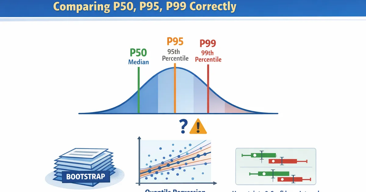
Percentiles and Latency: Comparing P50, P95, P99 Correctly
How to properly compare percentile metrics like latency P50, P95, and P99 across groups. Learn about bootstrap inference, quantile regression, and the pitfalls of naive percentile comparisons.
Quick Hits
- •Percentile standard errors aren't simple—bootstrap is the go-to method
- •Comparing P95/P99 requires much larger samples than comparing means
- •Quantile regression lets you model percentiles as functions of covariates
- •Don't just compare point estimates—quantify uncertainty properly
- •Mean latency can improve while P99 gets worse (and vice versa)
TL;DR
Percentile metrics (P50, P95, P99) are essential for latency and performance analysis, but comparing them requires care. Unlike means, percentile standard errors don't have simple formulas—use bootstrap for confidence intervals. High percentiles (P95, P99) need much larger samples because few observations fall in the tail. Quantile regression models percentiles as functions of covariates. This guide covers proper inference for percentile comparisons in product analytics.
Why Percentiles Matter
The Problem with Means
Latency distributions are typically:
- Right-skewed: Most requests are fast, some are slow
- Heavy-tailed: Occasional very slow requests
- Multi-modal: Different code paths have different speeds
Mean latency is dominated by the tail. One 10-second timeout in 1000 requests adds 10ms to mean latency—misleading when 99% of requests complete in <100ms.
What Percentiles Tell You
| Metric | Interpretation | Use Case |
|---|---|---|
| P50 (median) | Typical user experience | Dashboard headline |
| P75 | Upper-normal experience | Performance budgets |
| P95 | Worst 5% of users | SLA monitoring |
| P99 | Edge cases, one in 100 | Critical path alerts |
| P99.9 | Extreme tail | Debugging, capacity |
Different Percentiles, Different Stories
Scenario A: Mean improves, P99 worsens
- Old: P50=50ms, P99=500ms, Mean=80ms
- New: P50=45ms, P99=800ms, Mean=75ms
- Typical users faster, but worst cases much worse

Scenario B: Mean worsens, P99 improves
- Old: P50=50ms, P99=2000ms, Mean=100ms
- New: P50=55ms, P99=400ms, Mean=110ms
- Typical users slightly slower, but no more catastrophic delays
Bootstrap for Percentile Confidence Intervals
The Method
- Resample data with replacement (same size as original)
- Compute percentile on resampled data
- Repeat 1000+ times
- Use distribution of bootstrap percentiles for CI
Implementation
import numpy as np
from scipy import stats


def bootstrap_percentile_ci(data, percentile, n_bootstrap=2000, alpha=0.05):
    """
    Bootstrap confidence interval for a percentile.

    Parameters:
    -----------
    data : array-like
        Sample data
    percentile : float
        Percentile to estimate (0-100)
    n_bootstrap : int
        Number of bootstrap resamples
    alpha : float
        Significance level (0.05 for 95% CI)

    Returns:
    --------
    dict with point estimate and CI bounds
    """
    data = np.asarray(data)
    n = len(data)

    # Point estimate
    point_est = np.percentile(data, percentile)

    # Bootstrap
    bootstrap_percentiles = []
    for _ in range(n_bootstrap):
        resample = np.random.choice(data, size=n, replace=True)
        bootstrap_percentiles.append(np.percentile(resample, percentile))

    bootstrap_percentiles = np.array(bootstrap_percentiles)

    # Percentile method CI
    ci_lower = np.percentile(bootstrap_percentiles, 100 * alpha / 2)
    ci_upper = np.percentile(bootstrap_percentiles, 100 * (1 - alpha / 2))

    # BCa-corrected CI (more accurate)
    z0 = stats.norm.ppf(np.mean(bootstrap_percentiles < point_est))

    # Jackknife for acceleration
    jackknife_percentiles = []
    for i in range(n):
        jackknife_sample = np.delete(data, i)
        jackknife_percentiles.append(np.percentile(jackknife_sample, percentile))

    jackknife_percentiles = np.array(jackknife_percentiles)
    jack_mean = jackknife_percentiles.mean()
    acc = np.sum((jack_mean - jackknife_percentiles)**3) / \
          (6 * np.sum((jack_mean - jackknife_percentiles)**2)**1.5 + 1e-10)

    # BCa adjustments
    z_alpha_lower = stats.norm.ppf(alpha / 2)
    z_alpha_upper = stats.norm.ppf(1 - alpha / 2)

    a1 = stats.norm.cdf(z0 + (z0 + z_alpha_lower) / (1 - acc * (z0 + z_alpha_lower)))
    a2 = stats.norm.cdf(z0 + (z0 + z_alpha_upper) / (1 - acc * (z0 + z_alpha_upper)))

    ci_lower_bca = np.percentile(bootstrap_percentiles, 100 * a1)
    ci_upper_bca = np.percentile(bootstrap_percentiles, 100 * a2)

    return {
        'percentile': percentile,
        'point_estimate': point_est,
        'ci_lower': ci_lower,
        'ci_upper': ci_upper,
        'ci_lower_bca': ci_lower_bca,
        'ci_upper_bca': ci_upper_bca,
        'se': bootstrap_percentiles.std()
    }


# Example: Latency data
np.random.seed(42)

# Simulate log-normal latency (ms)
latency = np.random.lognormal(mean=4, sigma=0.8, size=5000)

# Compute CIs for multiple percentiles
for p in [50, 75, 95, 99]:
    result = bootstrap_percentile_ci(latency, p)
    print(f"P{p}: {result['point_estimate']:.1f}ms")
    print(f"  95% CI (percentile): ({result['ci_lower']:.1f}, {result['ci_upper']:.1f})")
    print(f"  95% CI (BCa):        ({result['ci_lower_bca']:.1f}, {result['ci_upper_bca']:.1f})")
    print(f"  Bootstrap SE: {result['se']:.1f}ms")
    print()
Comparing Percentiles Between Groups
Two-Sample Percentile Comparison
def compare_percentiles(group1, group2, percentile, n_bootstrap=2000, alpha=0.05):
    """
    Compare a percentile between two groups using bootstrap.

    Returns:
    --------
    dict with difference estimate, CI, and pseudo p-value
    """
    g1 = np.asarray(group1)
    g2 = np.asarray(group2)

    # Point estimates
    p1 = np.percentile(g1, percentile)
    p2 = np.percentile(g2, percentile)
    diff = p2 - p1
    ratio = p2 / p1 if p1 > 0 else np.inf

    # Bootstrap the difference
    bootstrap_diffs = []
    bootstrap_ratios = []

    for _ in range(n_bootstrap):
        resample1 = np.random.choice(g1, size=len(g1), replace=True)
        resample2 = np.random.choice(g2, size=len(g2), replace=True)

        bp1 = np.percentile(resample1, percentile)
        bp2 = np.percentile(resample2, percentile)

        bootstrap_diffs.append(bp2 - bp1)
        if bp1 > 0:
            bootstrap_ratios.append(bp2 / bp1)

    bootstrap_diffs = np.array(bootstrap_diffs)
    bootstrap_ratios = np.array(bootstrap_ratios)

    # CIs
    diff_ci = (np.percentile(bootstrap_diffs, 100 * alpha / 2),
               np.percentile(bootstrap_diffs, 100 * (1 - alpha / 2)))

    ratio_ci = (np.percentile(bootstrap_ratios, 100 * alpha / 2),
                np.percentile(bootstrap_ratios, 100 * (1 - alpha / 2)))

    # Pseudo p-value (proportion of bootstrap samples with opposite sign)
    if diff > 0:
        p_value = 2 * np.mean(bootstrap_diffs <= 0)
    else:
        p_value = 2 * np.mean(bootstrap_diffs >= 0)
    p_value = min(p_value, 1.0)

    return {
        'percentile': percentile,
        'group1': p1,
        'group2': p2,
        'difference': diff,
        'ratio': ratio,
        'diff_ci': diff_ci,
        'ratio_ci': ratio_ci,
        'p_value': p_value
    }


# Example: Compare latency between old and new version
np.random.seed(42)

old_version = np.random.lognormal(4, 0.8, 3000)  # Baseline
new_version = np.random.lognormal(3.95, 0.7, 3000)  # Slightly faster, less variable

print("Latency Comparison: Old vs. New Version")
print("=" * 60)

for p in [50, 95, 99]:
    result = compare_percentiles(old_version, new_version, p)
    print(f"\nP{p}:")
    print(f"  Old: {result['group1']:.1f}ms")
    print(f"  New: {result['group2']:.1f}ms")
    print(f"  Difference: {result['difference']:.1f}ms ({result['ratio']:.2%} of old)")
    print(f"  95% CI for difference: ({result['diff_ci'][0]:.1f}, {result['diff_ci'][1]:.1f})")
    print(f"  p-value: {result['p_value']:.4f}")
R Implementation
library(boot)

# Bootstrap CI for percentile
percentile_ci <- function(data, percentile, n_boot = 2000) {
    boot_fn <- function(data, indices) {
        quantile(data[indices], percentile / 100)
    }

    boot_result <- boot(data, boot_fn, R = n_boot)
    ci <- boot.ci(boot_result, type = "bca")

    list(
        estimate = quantile(data, percentile / 100),
        ci_lower = ci$bca[4],
        ci_upper = ci$bca[5]
    )
}

# Compare percentiles
compare_percentiles <- function(group1, group2, percentile, n_boot = 2000) {
    # Bootstrap difference
    boot_fn <- function(data, indices) {
        n1 <- length(group1)
        combined <- c(group1, group2)
        resample <- combined[indices]
        g1 <- resample[1:n1]
        g2 <- resample[(n1+1):length(resample)]
        quantile(g2, percentile/100) - quantile(g1, percentile/100)
    }

    combined <- c(group1, group2)
    indices <- 1:length(combined)

    # Simple percentile bootstrap
    diffs <- replicate(n_boot, {
        s1 <- sample(group1, replace = TRUE)
        s2 <- sample(group2, replace = TRUE)
        quantile(s2, percentile/100) - quantile(s1, percentile/100)
    })

    list(
        diff = quantile(group2, percentile/100) - quantile(group1, percentile/100),
        ci = quantile(diffs, c(0.025, 0.975))
    )
}
Sample Size Considerations
Why High Percentiles Need More Data
To estimate P99, you need observations above the 99th percentile. With n samples:
- Expected observations above P99:
- With : ~10 observations define P99
- With : ~1 observation—huge uncertainty
Effective Sample Size
| Percentile | Effective Sample Size | Multiplier vs. Mean |
|---|---|---|
| P50 | ||
| P75 | ||
| P90 | ||
| P95 | ||
| P99 |
Sample Size Calculation
def sample_size_for_percentile(percentile, desired_se_ratio, pilot_data):
    """
    Estimate sample size needed for desired precision on a percentile.

    Parameters:
    -----------
    percentile : float
        Target percentile (0-100)
    desired_se_ratio : float
        Desired SE as fraction of point estimate
    pilot_data : array
        Pilot data for variance estimation

    Returns:
    --------
    Estimated required sample size
    """
    # Bootstrap to estimate SE at pilot sample size
    n_pilot = len(pilot_data)
    current_result = bootstrap_percentile_ci(pilot_data, percentile, n_bootstrap=1000)

    current_se = current_result['se']
    point_est = current_result['point_estimate']
    current_se_ratio = current_se / point_est

    # SE scales roughly as 1/sqrt(n) for percentiles
    # Required n = pilot_n * (current_se_ratio / desired_se_ratio)^2
    required_n = n_pilot * (current_se_ratio / desired_se_ratio) ** 2

    return {
        'pilot_n': n_pilot,
        'pilot_se_ratio': current_se_ratio,
        'required_n': int(np.ceil(required_n)),
        'point_estimate': point_est,
        'current_se': current_se
    }


# Example: How much data for 10% precision on P99?
np.random.seed(42)
pilot = np.random.lognormal(4, 0.8, 500)

for p in [50, 95, 99]:
    result = sample_size_for_percentile(p, desired_se_ratio=0.10, pilot_data=pilot)
    print(f"P{p}:")
    print(f"  Pilot SE ratio: {result['pilot_se_ratio']:.1%}")
    print(f"  Required n for 10% precision: {result['required_n']:,}")
    print()
Quantile Regression
Beyond Simple Comparisons
Quantile regression models percentiles as functions of covariates:
Where τ is the quantile (0.5 for median, 0.95 for P95, etc.).
Why Use Quantile Regression?
- Multiple covariates: Control for confounders
- Different effects at different quantiles: Treatment may help P50 but hurt P99
- Full distributional picture: Model entire distribution, not just mean
Implementation
import statsmodels.api as sm
from statsmodels.regression.quantile_regression import QuantReg


def fit_quantile_regression(X, y, quantiles=[0.5, 0.75, 0.95, 0.99]):
    """
    Fit quantile regression at multiple quantiles.

    Parameters:
    -----------
    X : array
        Covariates (with constant)
    y : array
        Response variable
    quantiles : list
        Quantiles to estimate

    Returns:
    --------
    dict of fitted models and summaries
    """
    results = {}

    for q in quantiles:
        model = QuantReg(y, X)
        fitted = model.fit(q=q)
        results[q] = {
            'model': fitted,
            'params': fitted.params,
            'conf_int': fitted.conf_int(),
            'pvalues': fitted.pvalues
        }

    return results


# Example: Latency vs. request size and treatment
np.random.seed(42)
n = 2000

# Covariates
treatment = np.random.binomial(1, 0.5, n)
request_size = np.random.exponential(100, n)  # KB

# Latency: treatment reduces median but increases variance
base_latency = 50 + 0.5 * request_size
treatment_effect_location = -10 * treatment  # Faster median
treatment_effect_scale = 0.5 * treatment  # More variance in treatment
noise = np.random.exponential(20 + 20 * treatment, n)

latency = base_latency + treatment_effect_location + noise
latency = np.maximum(latency, 1)  # Floor at 1ms

# Fit quantile regression
X = sm.add_constant(np.column_stack([treatment, request_size]))
qr_results = fit_quantile_regression(X, latency)

print("Quantile Regression: Latency ~ Treatment + Request Size")
print("=" * 70)

for q, result in qr_results.items():
    print(f"\nQuantile {q} (P{int(q*100)}):")
    print(f"  Intercept: {result['params'][0]:.2f}")
    print(f"  Treatment effect: {result['params'][1]:.2f}ms")
    ci = result['conf_int'].loc['x1']
    print(f"    95% CI: ({ci[0]:.2f}, {ci[1]:.2f})")
    print(f"    p-value: {result['pvalues'][1]:.4f}")
    print(f"  Request size effect: {result['params'][2]:.3f}ms per KB")
R: Quantile Regression
library(quantreg)

# Fit quantile regression
model_p50 <- rq(latency ~ treatment + request_size, data = data, tau = 0.50)
model_p95 <- rq(latency ~ treatment + request_size, data = data, tau = 0.95)
model_p99 <- rq(latency ~ treatment + request_size, data = data, tau = 0.99)

# Summary with bootstrap CIs
summary(model_p95, se = "boot")

# Fit multiple quantiles at once
model_multi <- rq(latency ~ treatment + request_size,
                   data = data,
                   tau = c(0.25, 0.50, 0.75, 0.90, 0.95, 0.99))
summary(model_multi)

# Plot quantile process
plot(summary(model_multi))
Visualizing Percentile Comparisons
import matplotlib.pyplot as plt


def plot_percentile_comparison(group1, group2, labels=['Group 1', 'Group 2'],
                                percentiles=[50, 75, 90, 95, 99]):
    """
    Visualize percentile comparison between two groups.
    """
    fig, axes = plt.subplots(1, 2, figsize=(14, 5))

    # Left: Percentile plot with CIs
    ax1 = axes[0]
    x = np.arange(len(percentiles))
    width = 0.35

    p1_vals = []
    p1_errs = []
    p2_vals = []
    p2_errs = []

    for p in percentiles:
        r1 = bootstrap_percentile_ci(group1, p, n_bootstrap=1000)
        r2 = bootstrap_percentile_ci(group2, p, n_bootstrap=1000)
        p1_vals.append(r1['point_estimate'])
        p1_errs.append([r1['point_estimate'] - r1['ci_lower'],
                        r1['ci_upper'] - r1['point_estimate']])
        p2_vals.append(r2['point_estimate'])
        p2_errs.append([r2['point_estimate'] - r2['ci_lower'],
                        r2['ci_upper'] - r2['point_estimate']])

    p1_errs = np.array(p1_errs).T
    p2_errs = np.array(p2_errs).T

    ax1.bar(x - width/2, p1_vals, width, yerr=p1_errs, label=labels[0],
            capsize=5, alpha=0.8)
    ax1.bar(x + width/2, p2_vals, width, yerr=p2_errs, label=labels[1],
            capsize=5, alpha=0.8)

    ax1.set_xlabel('Percentile')
    ax1.set_ylabel('Latency (ms)')
    ax1.set_title('Percentile Comparison with 95% CIs')
    ax1.set_xticks(x)
    ax1.set_xticklabels([f'P{p}' for p in percentiles])
    ax1.legend()

    # Right: Distribution comparison
    ax2 = axes[1]
    ax2.hist(group1, bins=50, alpha=0.5, label=labels[0], density=True)
    ax2.hist(group2, bins=50, alpha=0.5, label=labels[1], density=True)

    # Add percentile markers
    for p in [50, 95, 99]:
        ax2.axvline(np.percentile(group1, p), color='C0', linestyle='--', alpha=0.7)
        ax2.axvline(np.percentile(group2, p), color='C1', linestyle='--', alpha=0.7)

    ax2.set_xlabel('Latency (ms)')
    ax2.set_ylabel('Density')
    ax2.set_title('Distribution with Percentile Markers')
    ax2.legend()

    plt.tight_layout()
    return fig


# Example
np.random.seed(42)
old = np.random.lognormal(4, 0.8, 2000)
new = np.random.lognormal(3.9, 0.6, 2000)

fig = plot_percentile_comparison(old, new, labels=['Old', 'New'])
plt.show()
Common Pitfalls
1. Ignoring Uncertainty
Wrong: "P99 improved from 500ms to 450ms" Right: "P99 improved from 500ms to 450ms (95% CI: 380-520ms)"
2. Wrong Sample Size Assumptions
Wrong: "n=1000 per group is enough" Right: Calculate required n based on target percentile
3. Comparing Single Points
Wrong: Compare only P99 Right: Look at multiple percentiles—effects may differ
4. Assuming Same Effect Everywhere
Wrong: "Treatment improved latency" (based on mean or P50) Right: Check if improvement is consistent across distribution
Related Methods
- Metric Distributions (Pillar) - Full distributions overview
- Bootstrap for Heavy-Tailed Metrics - Bootstrap deep dive
- Comparing Medians - Median-specific tests
- Mann-Whitney U - Rank-based comparisons
Key Takeaway
Percentile metrics require different statistical treatment than means. P50 captures typical experience; P95/P99 capture tail behavior. Bootstrap is the standard method for percentile confidence intervals—don't just compare point estimates. High percentiles need much larger samples: P99 comparisons require roughly 50× the data of mean comparisons. Quantile regression extends to multiple covariates and reveals if effects differ across the distribution. Always check multiple percentiles—improving the median while making the tail worse (or vice versa) is common.
References
- https://doi.org/10.1007/978-0-387-98141-3
- https://doi.org/10.1111/j.1467-9868.2005.00510.x
- https://www.jstatsoft.org/article/view/v027i02
- Koenker, R. (2005). *Quantile Regression*. Cambridge University Press.
- Efron, B., & Tibshirani, R. J. (1993). *An Introduction to the Bootstrap*. Chapman & Hall.
- Hyndman, R. J., & Fan, Y. (1996). Sample quantiles in statistical packages. *The American Statistician*, 50(4), 361-365.
Frequently Asked Questions
Why not just compare means for latency?
How do I get confidence intervals for percentiles?
How much data do I need to compare P99?
Key Takeaway
Percentile metrics like P50, P95, and P99 require different statistical treatment than means. Bootstrap confidence intervals are the workhorse for inference. Quantile regression extends to multiple covariates. Sample sizes must be much larger for high percentiles—P99 comparisons need roughly 100× the data of mean comparisons. Always report uncertainty, and consider whether the percentile you're comparing actually answers your business question.