Contents
Comparing Medians: Statistical Tests and Better Options
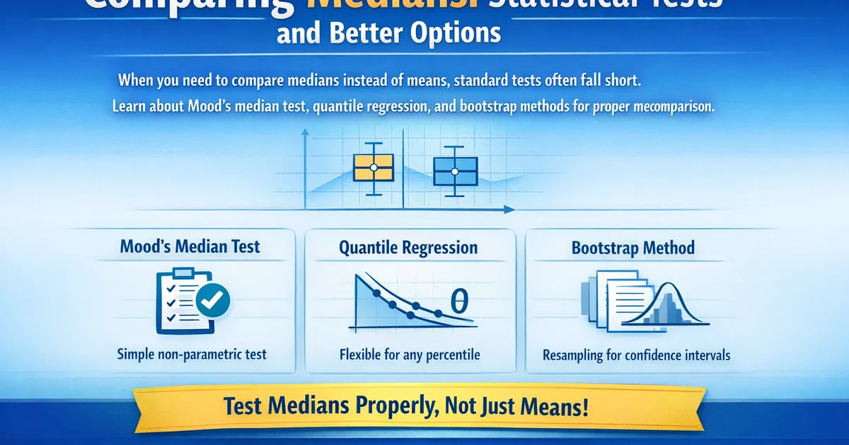
When you need to compare medians instead of means, standard tests often fall short. Learn about Mood's median test, quantile regression, and bootstrap methods for proper median comparison.
Quick Hits
- •Mann-Whitney doesn't test medians—it tests stochastic dominance
- •Mood's median test has low power but actually tests what it claims
- •Quantile regression is more flexible and extends to any percentile
- •Bootstrap is often the simplest approach for median confidence intervals
TL;DR
Comparing medians is harder than it looks. Mann-Whitney doesn't actually test medians (it tests stochastic dominance). Mood's median test actually tests medians but has low power. Quantile regression offers flexibility. Bootstrap provides straightforward confidence intervals. Choose based on your actual question and data.
Why Medians?
Medians matter when:
- Outliers dominate: A few extreme values pull the mean far from "typical"
- Skewed distributions: Mean and median differ substantially
- Ordinal data: Arithmetic mean isn't meaningful
- "Typical user" matters: You care about the 50th percentile experience
But consider: for many business metrics, totals matter. Total revenue = mean × users, not median × users. Medians can hide important variation.
Method 1: Mood's Median Test
The only classic test that actually tests whether medians differ.
How It Works
- Find the grand median (median of all observations combined)
- Count how many observations in each group fall above/below the grand median
- Test whether these counts differ between groups (chi-square test)
from scipy import stats
import numpy as np

def moods_median_test(group1, group2):
    """
    Mood's median test for comparing medians.
    """
    stat, p_value, grand_median, table = stats.median_test(group1, group2)

    return {
        'statistic': stat,
        'p_value': p_value,
        'grand_median': grand_median,
        'contingency_table': table,
        'group1_median': np.median(group1),
        'group2_median': np.median(group2)
    }


# Example
np.random.seed(42)
group1 = np.random.exponential(10, 100)
group2 = np.random.exponential(15, 100)

result = moods_median_test(group1, group2)
print(f"Group 1 median: {result['group1_median']:.2f}")
print(f"Group 2 median: {result['group2_median']:.2f}")
print(f"P-value: {result['p_value']:.4f}")
R Implementation
# Mood's median test in R
library(RVAideMemoire)
mood.medtest(value ~ group, data = df)

# Or using base R approach
grand_median <- median(c(group1, group2))
table <- matrix(c(
  sum(group1 > grand_median), sum(group1 <= grand_median),
  sum(group2 > grand_median), sum(group2 <= grand_median)
), nrow = 2, byrow = TRUE)
chisq.test(table)
Limitations
Low power: Mood's test only uses information about whether observations are above/below the median. It ignores how far above or below. This wastes information.
Ties at median: When observations equal the grand median, results depend on how ties are handled.
Large samples needed: Due to low power, you need substantial samples for reliable detection.
Method 2: Bootstrap
The most straightforward approach: resample to estimate the median difference and its uncertainty.
Implementation
import numpy as np

def bootstrap_median_comparison(group1, group2, n_bootstrap=10000, alpha=0.05):
    """
    Bootstrap comparison of medians.
    """
    observed_diff = np.median(group2) - np.median(group1)

    # Bootstrap distribution of difference
    diffs = []
    for _ in range(n_bootstrap):
        boot1 = np.random.choice(group1, size=len(group1), replace=True)
        boot2 = np.random.choice(group2, size=len(group2), replace=True)
        diffs.append(np.median(boot2) - np.median(boot1))

    diffs = np.array(diffs)

    # Percentile confidence interval
    ci_lower = np.percentile(diffs, 100 * alpha / 2)
    ci_upper = np.percentile(diffs, 100 * (1 - alpha / 2))

    # Bootstrap p-value via permutation
    combined = np.concatenate([group1, group2])
    null_diffs = []
    for _ in range(n_bootstrap):
        np.random.shuffle(combined)
        perm1 = combined[:len(group1)]
        perm2 = combined[len(group1):]
        null_diffs.append(np.median(perm2) - np.median(perm1))

    null_diffs = np.array(null_diffs)
    p_value = np.mean(np.abs(null_diffs) >= np.abs(observed_diff))

    return {
        'median_group1': np.median(group1),
        'median_group2': np.median(group2),
        'median_difference': observed_diff,
        'ci_95': (ci_lower, ci_upper),
        'p_value': p_value
    }


# Example
result = bootstrap_median_comparison(group1, group2)
print(f"Median difference: {result['median_difference']:.2f}")
print(f"95% CI: [{result['ci_95'][0]:.2f}, {result['ci_95'][1]:.2f}]")
print(f"P-value: {result['p_value']:.4f}")
Advantages
- Simple and intuitive: Directly estimates what you want
- Honest uncertainty: CI width reflects actual sampling variability
- Flexible: Works for any percentile, not just median
- No distributional assumptions: Works for any data
Considerations
- Computational cost: Requires many resamples (10,000+)
- Discrete medians: With discrete data, bootstrap medians can be jumpy
- Small samples: Performance degrades with very small n
Method 3: Quantile Regression
Regression framework for estimating conditional quantiles. More powerful than Mood's test and extends to include covariates.
Python Implementation
import statsmodels.formula.api as smf
import pandas as pd
import numpy as np

def quantile_regression_comparison(group1, group2, quantile=0.5):
    """
    Compare groups using quantile regression.
    """
    # Create dataframe
    df = pd.DataFrame({
        'value': np.concatenate([group1, group2]),
        'treatment': [0] * len(group1) + [1] * len(group2)
    })

    # Fit quantile regression
    model = smf.quantreg('value ~ treatment', df)
    result = model.fit(q=quantile)

    return {
        'quantile': quantile,
        'coefficient': result.params['treatment'],
        'std_error': result.bse['treatment'],
        'p_value': result.pvalues['treatment'],
        'ci_lower': result.conf_int().loc['treatment', 0],
        'ci_upper': result.conf_int().loc['treatment', 1]
    }


# Example: compare medians
result = quantile_regression_comparison(group1, group2, quantile=0.5)
print(f"Median difference estimate: {result['coefficient']:.2f}")
print(f"95% CI: [{result['ci_lower']:.2f}, {result['ci_upper']:.2f}]")
print(f"P-value: {result['p_value']:.4f}")
R Implementation
library(quantreg)

df <- data.frame(
  value = c(group1, group2),
  treatment = c(rep(0, length(group1)), rep(1, length(group2)))
)

# Median regression
fit <- rq(value ~ treatment, data = df, tau = 0.5)
summary(fit)
Advantages
- More power than Mood's: Uses full information about values
- Handles covariates: Can adjust for confounders
- Any quantile: Estimate 25th, 75th percentile differences too
- Proper inference: Standard errors and CIs
Comparing Multiple Quantiles
def multi_quantile_comparison(group1, group2, quantiles=[0.25, 0.5, 0.75]):
    """
    Compare groups across multiple quantiles.
    """
    df = pd.DataFrame({
        'value': np.concatenate([group1, group2]),
        'treatment': [0] * len(group1) + [1] * len(group2)
    })

    results = []
    for q in quantiles:
        model = smf.quantreg('value ~ treatment', df)
        fit = model.fit(q=q)
        results.append({
            'quantile': q,
            'effect': fit.params['treatment'],
            'p_value': fit.pvalues['treatment']
        })

    return pd.DataFrame(results)


# Compare across distribution
comparison = multi_quantile_comparison(group1, group2)
print(comparison)
Why Mann-Whitney Doesn't Test Medians
A common misconception: "Mann-Whitney tests whether medians differ."
The Truth
Mann-Whitney tests whether P(X > Y) = 0.5. This equals testing medians ONLY if you assume:
- Both distributions have the same shape
- One is just a shifted version of the other
Without this assumption, Mann-Whitney and median tests can disagree:
# Example where Mann-Whitney and median tests disagree
np.random.seed(123)

# Group 1: Normal(0, 1)
group1 = np.random.normal(0, 1, 200)

# Group 2: Same median (0), but different shape
group2 = np.concatenate([
    np.random.uniform(-3, 0, 100),   # Below median
    np.random.uniform(0, 0.5, 100)   # Above median but close
])

print(f"Group 1 median: {np.median(group1):.2f}")
print(f"Group 2 median: {np.median(group2):.2f}")

# Mood's median test: no difference
mood_stat, mood_p, _, _ = stats.median_test(group1, group2)
print(f"\nMood's test p-value: {mood_p:.4f}")

# Mann-Whitney: significant difference!
mw_stat, mw_p = stats.mannwhitneyu(group1, group2)
print(f"Mann-Whitney p-value: {mw_p:.4f}")
Medians are nearly equal, but Mann-Whitney detects that the distributions differ in stochastic ordering.
Decision Guide
| Situation | Recommended Method |
|---|---|
| Simple median comparison, large samples | Mood's median test or bootstrap |
| Median comparison with covariates | Quantile regression |
| Want confidence interval | Bootstrap or quantile regression |
| Small samples | Bootstrap |
| Multiple quantiles | Quantile regression |
| Quick robustness check | Mann-Whitney (knowing its limitations) |
Practical Example
# A/B test with revenue data
np.random.seed(42)

# Control: typical revenue distribution
control = np.concatenate([
    np.zeros(500),  # Non-purchasers
    np.random.exponential(50, 400),  # Regular purchasers
    np.random.exponential(500, 100)  # Whales
])

# Treatment: shifts some non-purchasers to purchasers
treatment = np.concatenate([
    np.zeros(400),  # Fewer non-purchasers
    np.random.exponential(50, 500),  # More regular purchasers
    np.random.exponential(500, 100)  # Same whales
])

print("Means:")
print(f"  Control: ${np.mean(control):.2f}")
print(f"  Treatment: ${np.mean(treatment):.2f}")

print("\nMedians:")
print(f"  Control: ${np.median(control):.2f}")
print(f"  Treatment: ${np.median(treatment):.2f}")

# Bootstrap comparison of medians
result = bootstrap_median_comparison(control, treatment)
print(f"\nMedian difference: ${result['median_difference']:.2f}")
print(f"95% CI: [${result['ci_95'][0]:.2f}, ${result['ci_95'][1]:.2f}]")
Related Methods
- Picking the Right Test to Compare Two Groups — Complete decision framework
- Mann-Whitney U Test: What It Actually Tests — Why it's not a median test
- Non-Normal Metrics: Bootstrap, Mann-Whitney, and Log Transforms — Broader context
Key Takeaway
If you want to compare medians, use a method that actually tests medians: bootstrap for simplicity, quantile regression for flexibility and covariates, or Mood's median test for a basic significance test. Mann-Whitney tests something different (stochastic dominance) despite common misconception. Always be clear about whether median is the right summary—for many business metrics, mean matters more.
References
- https://www.jstor.org/stable/2684360
- https://www.jstor.org/stable/2332641
- Koenker, R., & Bassett Jr, G. (1978). Regression quantiles. *Econometrica*, 46(1), 33-50.
- Mood, A. M. (1954). On the asymptotic efficiency of certain nonparametric two-sample tests. *The Annals of Mathematical Statistics*, 25(3), 514-522.
- Divine, G. W., Norton, H. J., Barón, A. E., & Juarez-Colunga, E. (2018). The Wilcoxon-Mann-Whitney procedure fails as a test of medians. *The American Statistician*, 72(3), 278-286.
Frequently Asked Questions
Doesn't Mann-Whitney test whether medians differ?
When should I compare medians instead of means?
What's the best test for comparing medians?
Key Takeaway
If you want to compare medians, use a method that actually tests medians: bootstrap, quantile regression, or Mood's median test. Mann-Whitney tests something different (stochastic dominance) despite common misconception.