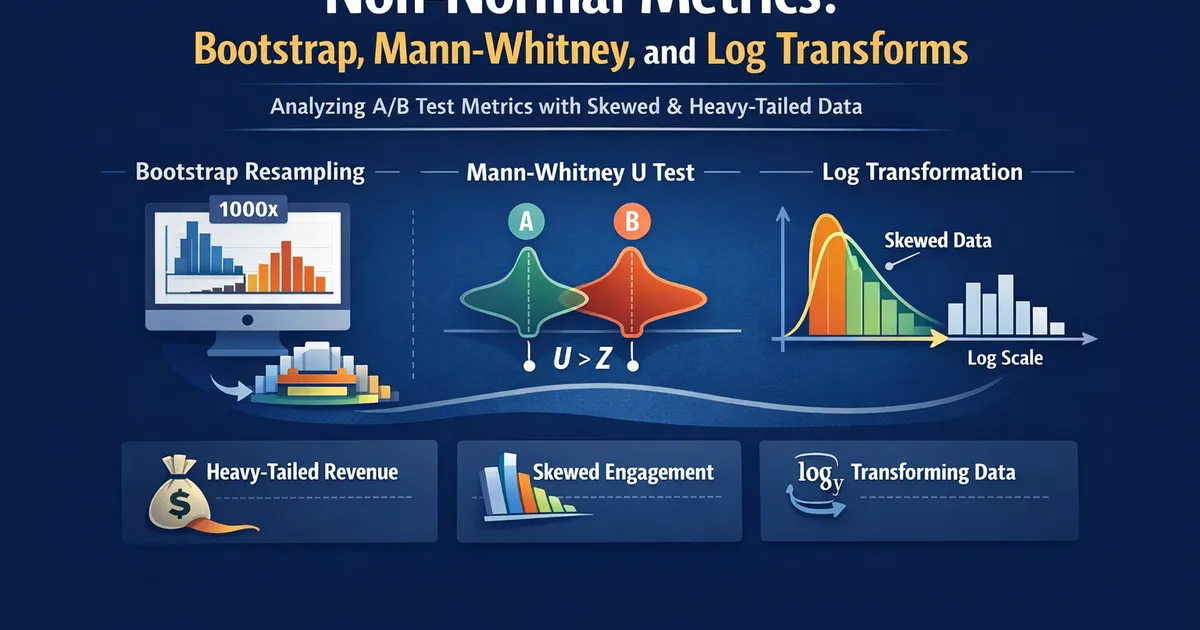
Non-Normal Metrics: Bootstrap, Mann-Whitney, and Log Transforms

TL;DR

Product metrics are messy—revenue has whales, session times have zombies, engagement has power users. These distributions violate normality assumptions. But don't panic: t-tests are robust to moderate non-normality with large samples. When they're not enough, bootstrap methods handle anything. Mann-Whitney tests a different question (dominance, not means), and log transforms change what you're measuring. Choose based on your actual question.

When Non-Normality Matters

The Central Limit Theorem Saves You (Usually)

The t-test assumes the sampling distribution of the mean is normal. Thanks to the Central Limit Theorem, this is approximately true for large samples even when individual observations are non-normal.

Rules of thumb:

• n > 30 per group: t-test is robust to moderate skew
• n > 100 per group: t-test handles substantial skew
• n > 1000 per group: t-test works for almost anything

import numpy as np
from scipy import stats

def simulate_ttest_robustness(distribution, n_per_group, n_simulations=10000):
    """
    Simulate t-test under non-normal data to check Type I error.
    """
    significant = 0

    for _ in range(n_simulations):
        # Generate from non-normal distribution (same for both groups = null true)
        control = distribution(n_per_group)
        treatment = distribution(n_per_group)

        _, p = stats.ttest_ind(control, treatment)
        if p < 0.05:
            significant += 1

    return significant / n_simulations


# Test with exponential distribution (very skewed)
exponential = lambda n: np.random.exponential(1, n)

for n in [10, 30, 100, 1000]:
    fp_rate = simulate_ttest_robustness(exponential, n)
    print(f"n={n:4d}: False positive rate = {fp_rate:.3f} (should be ~0.05)")

# Output (typical):
# n=  10: False positive rate = 0.062 (elevated)
# n=  30: False positive rate = 0.052 (close)
# n= 100: False positive rate = 0.050 (good)
# n=1000: False positive rate = 0.050 (excellent)

When You Should Worry

1. Small samples: n < 30 per group with obvious non-normality
2. Extreme outliers: A few values 100x larger than typical
3. Heavy tails: Distributions where extreme values dominate the mean
4. Bimodal/multimodal: Distinct subpopulations in your data

Method 1: Bootstrap

Bootstrap resampling is the universal solution for non-normal data. It makes no distributional assumptions and works for any statistic.

The Idea

1. Resample your data with replacement, creating many "bootstrap samples"
2. Compute your statistic on each bootstrap sample
3. Use the distribution of bootstrap statistics for inference

Python Implementation

import numpy as np
from scipy import stats

def bootstrap_mean_diff(control, treatment, n_bootstrap=10000, alpha=0.05):
    """
    Bootstrap confidence interval for difference in means.
    """
    diffs = []

    for _ in range(n_bootstrap):
        c_sample = np.random.choice(control, size=len(control), replace=True)
        t_sample = np.random.choice(treatment, size=len(treatment), replace=True)
        diffs.append(np.mean(t_sample) - np.mean(c_sample))

    diffs = np.array(diffs)

    # Percentile confidence interval
    ci_lower = np.percentile(diffs, 100 * alpha / 2)
    ci_upper = np.percentile(diffs, 100 * (1 - alpha / 2))

    # P-value (two-sided test of no difference)
    observed_diff = np.mean(treatment) - np.mean(control)
    # Null distribution: shift treatment to have same mean as control
    treatment_null = treatment - np.mean(treatment) + np.mean(control)

    null_diffs = []
    for _ in range(n_bootstrap):
        c_sample = np.random.choice(control, size=len(control), replace=True)
        t_sample = np.random.choice(treatment_null, size=len(treatment_null), replace=True)
        null_diffs.append(np.mean(t_sample) - np.mean(c_sample))

    null_diffs = np.array(null_diffs)
    p_value = np.mean(np.abs(null_diffs) >= np.abs(observed_diff))

    return {
        'difference': observed_diff,
        'ci_lower': ci_lower,
        'ci_upper': ci_upper,
        'p_value': p_value
    }


# Example with heavy-tailed revenue data
np.random.seed(42)
# Simulate revenue: most users spend $0-50, some spend $500+
control = np.concatenate([
    np.random.exponential(10, 900),  # Regular users
    np.random.exponential(200, 100)  # Whales
])
treatment = np.concatenate([
    np.random.exponential(11, 900),  # 10% lift for regular users
    np.random.exponential(200, 100)  # Same whales
])

result = bootstrap_mean_diff(control, treatment)
print(f"Difference: ${result['difference']:.2f}")
print(f"95% CI: [${result['ci_lower']:.2f}, ${result['ci_upper']:.2f}]")
print(f"P-value: {result['p_value']:.4f}")

R Implementation

library(boot)

# Bootstrap function for mean difference
mean_diff <- function(data, indices) {
  d <- data[indices, ]
  return(mean(d[d$group == "treatment", "value"]) -
         mean(d[d$group == "control", "value"]))
}

# Create data frame
df <- data.frame(
  value = c(control, treatment),
  group = rep(c("control", "treatment"), c(length(control), length(treatment)))
)

# Run bootstrap
boot_result <- boot(df, mean_diff, R = 10000)
boot.ci(boot_result, type = "perc")

When Bootstrap Shines

• Complex metrics: Ratios, percentiles, medians
• Heavily skewed data: Revenue, session duration
• Small samples: When CLT may not apply
• Non-standard statistics: Any function of your data

Bootstrap Limitations

• Computationally expensive: 10,000+ resamples needed
• Assumes representative sample: Garbage in, garbage out
• Doesn't fix selection bias: Bootstrap estimates uncertainty, not bias
• Heavy tails need more resamples: Rare outliers need more samples to capture

Method 2: Mann-Whitney U Test

Mann-Whitney (also called Wilcoxon rank-sum) is a non-parametric test that doesn't assume normality. But beware: it tests something different than the t-test.

What Mann-Whitney Tests

Mann-Whitney tests stochastic dominance: the probability that a randomly selected treatment observation exceeds a randomly selected control observation.

This is NOT the same as "means differ." Two groups can have:

• Same mean but different Mann-Whitney result (different shape)
• Different mean but same Mann-Whitney result (symmetric shifts)

Python Implementation

from scipy import stats

def mann_whitney_test(control, treatment):
    """
    Mann-Whitney U test for stochastic dominance.
    """
    stat, p_value = stats.mannwhitneyu(control, treatment, alternative='two-sided')

    # Probability that treatment > control
    n1, n2 = len(control), len(treatment)
    prob_treatment_greater = stat / (n1 * n2)

    return {
        'u_statistic': stat,
        'p_value': p_value,
        'prob_treatment_greater': prob_treatment_greater
    }


result = mann_whitney_test(control, treatment)
print(f"P-value: {result['p_value']:.4f}")
print(f"P(treatment > control): {result['prob_treatment_greater']:.3f}")

R Implementation

wilcox.test(treatment, control)

When to Use Mann-Whitney

• Testing whether treatment "tends to be higher" (not means)
• Ordinal data (rankings, Likert scales)
• When the business question is about typical values, not totals
• As a robustness check alongside t-test

When NOT to Use Mann-Whitney

• When you specifically care about means (use bootstrap instead)
• When you'll report effect size as mean difference
• When business impact is calculated from totals (revenue per user × users = total revenue)

Method 3: Log Transform

Log-transforming skewed data can make it more normal, enabling standard parametric tests.

What Log Transform Tests

After log transform, the t-test compares log-means. Back-transformed, this is the ratio of geometric means:

$$\text{Geometric mean} = \exp(\text{mean of log values})$$

import numpy as np

# Example
values = [1, 2, 4, 8, 16]

arithmetic_mean = np.mean(values)  # 6.2
geometric_mean = np.exp(np.mean(np.log(values)))  # 4.0

print(f"Arithmetic mean: {arithmetic_mean}")
print(f"Geometric mean: {geometric_mean}")

The geometric mean is always ≤ arithmetic mean, with equality only when all values are identical.

When Log Transform Is Appropriate

Multiplicative effects: If treatment causes a percentage change (10% lift for everyone), log-scale makes sense.

# Multiplicative effect example
control = np.random.exponential(100, 1000)
treatment = control * 1.1  # 10% lift for everyone

# Raw t-test
_, p_raw = stats.ttest_ind(control, treatment)

# Log t-test
_, p_log = stats.ttest_ind(np.log(control), np.log(treatment))

print(f"Raw p-value: {p_raw:.4f}")
print(f"Log p-value: {p_log:.4f}")
# Log test will be more powerful here

Ratio metrics: Click-through rates, conversion rates often benefit from logit transform (log-odds).

When Log Transform Is Problematic

Zeros: log(0) = -∞. Common workaround is log(x + 1), but this changes the interpretation.

# Handling zeros
values_with_zeros = [0, 0, 0, 1, 2, 5, 10, 100]

# Option 1: log(x + 1)
log_transformed = np.log(np.array(values_with_zeros) + 1)

# Option 2: Exclude zeros and analyze separately
non_zero = [v for v in values_with_zeros if v > 0]
log_non_zero = np.log(non_zero)

# Option 3: Two-part model (see related article)

Additive effects: If treatment adds a fixed amount (everyone gets $5 off), log-scale obscures this.

Business interpretation: If stakeholders need arithmetic mean (total revenue / users), log-transformed results are confusing.

Decision Framework

Is your sample large (n > 100 per group)?
├── Yes → Is the question about means?
│   ├── Yes → T-test is probably fine (robust to non-normality)
│   └── No → Use method matching your question
└── No → Are there extreme outliers or heavy tails?
    ├── Yes → Bootstrap or consider trimmed means
    └── No → T-test might still work; consider bootstrap for confirmation

What are you trying to test?
├── Mean difference → T-test or bootstrap
├── Median difference → Bootstrap or quantile regression
├── "Tends to be higher" → Mann-Whitney
├── Multiplicative effect → Log transform + t-test
└── Complex metric → Bootstrap

Practical Recommendation

For most A/B tests:

1. Default: Welch's t-test (handles unequal variances, robust to moderate non-normality)
2. Validate: Check histogram of your metric. Extreme skew? Run bootstrap as confirmation
3. Report: If t-test and bootstrap agree, report t-test (simpler). If they disagree, investigate why and report bootstrap

Handling Outliers

Outliers disproportionately affect means. Options:

Winsorization

Cap extreme values at a percentile:

from scipy.stats import mstats

def winsorize(data, limits=(0.01, 0.01)):
    """Winsorize at 1st and 99th percentile by default."""
    return mstats.winsorize(data, limits=limits)

# Cap at 1st and 99th percentile
control_wins = winsorize(control)
treatment_wins = winsorize(treatment)

Trimmed Means

Exclude extreme values from mean calculation:

from scipy.stats import trim_mean

# 10% trimmed mean (exclude top and bottom 5%)
control_trimmed = trim_mean(control, 0.05)
treatment_trimmed = trim_mean(treatment, 0.05)

# Yuen's test for trimmed mean difference
from scipy.stats import mstats
stat, p = mstats.ttest_ind(control, treatment, trim=0.1)

When to Use

• Pre-registered rule: Decide before seeing data
• Document clearly: Report both raw and trimmed results
• Understand impact: Trimming can change your answer substantially

Related Methods

• A/B Testing Statistical Methods for Product Teams — Complete guide to A/B testing
• Why Revenue Is Hard: Log-Normal and Heavy Tails — Deep dive into revenue distributions
• Bootstrap for Heavy-Tailed Metrics — Advanced bootstrap techniques

Frequently Asked Questions

Q: Should I test for normality before choosing a method? A: Formal normality tests are nearly useless. With large samples, they reject normality for tiny deviations that don't affect inference. With small samples, they lack power to detect meaningful non-normality. Instead, look at histograms and use domain knowledge.

Q: Is median better than mean for skewed data? A: Median is more robust to outliers but answers a different question. If business impact is calculated from totals (mean × users), you need mean. Median tells you about the typical user.

Q: Can I use both t-test and Mann-Whitney? A: Yes, as a robustness check. If they give different conclusions, investigate why (likely different questions being answered or extreme outliers affecting the mean).

Q: How many bootstrap resamples do I need? A: 10,000 is standard for confidence intervals, 1,000 might suffice for point estimates. For p-values, use at least 10,000.

Key Takeaway

For most A/B tests with reasonable sample sizes, the t-test works fine despite non-normality. When it doesn't—small samples, extreme skew, or outliers—bootstrap is your Swiss Army knife. It handles any metric and gives honest confidence intervals. Use Mann-Whitney only when testing "tends to be higher" (stochastic dominance) rather than mean difference. And remember: log transforms change what you're testing.

References

- https://www.jstor.org/stable/2684360
- https://www.stat.berkeley.edu/~census/bootstrap.pdf
- Efron, B., & Tibshirani, R. J. (1993). *An Introduction to the Bootstrap*. Chapman & Hall/CRC.
- Lumley, T., Diehr, P., Emerson, S., & Chen, L. (2002). The importance of the normality assumption in large public health data sets. *Annual Review of Public Health*, 23(1), 151-169.
- Mann, H. B., & Whitney, D. R. (1947). On a test of whether one of two random variables is stochastically larger than the other. *The Annals of Mathematical Statistics*, 18(1), 50-60.