Contents
Delta Method vs. Bootstrap: When Each Is Appropriate
A practical guide to choosing between delta method and bootstrap for variance estimation. Learn when each approach excels, their assumptions, and how to implement both.
Quick Hits
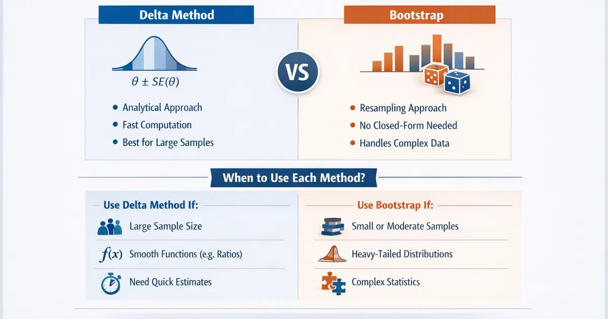
- •Delta method: fast, analytical, works well for large n and smooth functions
- •Bootstrap: flexible, no closed-form needed, handles complex statistics
- •Both should give similar results for well-behaved data—compare as sanity check
- •Heavy tails favor bootstrap; ratios with large n favor delta method
- •When in doubt, use both and report if they differ substantially
TL;DR
The delta method and bootstrap are two approaches to variance estimation for complex statistics. Delta method is analytical—fast and efficient for large samples with smooth functions of means. Bootstrap is computational—flexible and robust for complex statistics without closed-form variances. Both should give similar results for well-behaved data; when they disagree, investigate why. This guide helps you choose the right tool for your situation.
The Two Approaches
Delta Method
Core idea: Approximate a function of random variables using Taylor expansion.
For statistic where is a vector of sample means:
Where:
- = gradient of g evaluated at true means
- = covariance matrix of underlying variables
- = sample size
Example: For ratio :
Bootstrap
Core idea: Treat sample as population, resample to estimate sampling variability.
- Draw B resamples with replacement
- Compute statistic on each resample
- Use distribution of bootstrap statistics for inference
Example: For any statistic :
Quick Comparison
| Aspect | Delta Method | Bootstrap |
|---|---|---|
| Computation | Fast (analytical) | Slow (many resamples) |
| Assumptions | Large n, smooth function | Sample represents population |
| Flexibility | Need variance formula | Works for any statistic |
| Heavy tails | Can fail | More robust |
| Small samples | Can fail | Better (with caveats) |
| Implementation | Needs calculus | Straightforward |
Implementation Side-by-Side
import numpy as np
from scipy import stats


def delta_method_ratio(numerator, denominator):
    """
    Delta method SE for ratio of means.
    """
    n = len(numerator)

    mean_y = np.mean(numerator)
    mean_x = np.mean(denominator)
    ratio = mean_y / mean_x

    var_y = np.var(numerator, ddof=1)
    var_x = np.var(denominator, ddof=1)
    cov_xy = np.cov(numerator, denominator, ddof=1)[0, 1]

    var_ratio = (1 / mean_x**2) * (
        var_y - 2 * ratio * cov_xy + ratio**2 * var_x
    ) / n

    return {'estimate': ratio, 'se': np.sqrt(var_ratio)}


def bootstrap_ratio(numerator, denominator, n_bootstrap=5000):
    """
    Bootstrap SE for ratio of means.
    """
    n = len(numerator)
    ratio = np.sum(numerator) / np.sum(denominator)

    boot_ratios = []
    for _ in range(n_bootstrap):
        idx = np.random.choice(n, n, replace=True)
        boot_ratio = np.sum(numerator[idx]) / np.sum(denominator[idx])
        boot_ratios.append(boot_ratio)

    return {
        'estimate': ratio,
        'se': np.std(boot_ratios),
        'ci': np.percentile(boot_ratios, [2.5, 97.5])
    }


def compare_methods(numerator, denominator, n_bootstrap=5000):
    """
    Compare delta method and bootstrap for the same statistic.
    """
    delta_result = delta_method_ratio(numerator, denominator)
    boot_result = bootstrap_ratio(numerator, denominator, n_bootstrap)

    return {
        'delta': delta_result,
        'bootstrap': boot_result,
        'se_ratio': delta_result['se'] / boot_result['se'],
        'agreement': abs(delta_result['se'] - boot_result['se']) / boot_result['se'] < 0.1
    }


# Example: Well-behaved data
np.random.seed(42)
n = 1000
clicks = np.random.poisson(5, n)
impressions = np.random.poisson(50, n)

result = compare_methods(clicks, impressions)

print("Method Comparison: CTR with Well-Behaved Data")
print("=" * 50)
print(f"Sample size: {n}")
print(f"\nDelta Method:")
print(f"  CTR estimate: {result['delta']['estimate']:.4f}")
print(f"  SE: {result['delta']['se']:.6f}")
print(f"\nBootstrap:")
print(f"  CTR estimate: {result['bootstrap']['estimate']:.4f}")
print(f"  SE: {result['bootstrap']['se']:.6f}")
print(f"  95% CI: ({result['bootstrap']['ci'][0]:.4f}, {result['bootstrap']['ci'][1]:.4f})")
print(f"\nDelta/Bootstrap SE ratio: {result['se_ratio']:.3f}")
print(f"Methods agree (<10% difference): {result['agreement']}")
When Delta Method Excels
Large Samples
Delta method is asymptotically correct—as n → ∞, it converges to the true variance.
def show_delta_convergence():
    """
    Show delta method improves with sample size.
    """
    np.random.seed(42)

    true_ctr = 0.10
    n_simulations = 500

    sample_sizes = [100, 500, 1000, 5000]
    results = []

    for n in sample_sizes:
        delta_ses = []
        boot_ses = []

        for _ in range(n_simulations):
            impressions = np.random.poisson(50, n)
            clicks = np.random.binomial(impressions, true_ctr)

            delta_ses.append(delta_method_ratio(clicks, impressions)['se'])
            boot_ses.append(bootstrap_ratio(clicks, impressions, n_bootstrap=1000)['se'])

        results.append({
            'n': n,
            'delta_mean_se': np.mean(delta_ses),
            'boot_mean_se': np.mean(boot_ses),
            'delta_se_of_se': np.std(delta_ses),
            'boot_se_of_se': np.std(boot_ses)
        })

    print("Delta Method Performance by Sample Size")
    print("=" * 60)
    print(f"{'n':>8} {'Delta SE':>12} {'Boot SE':>12} {'Ratio':>10}")
    print("-" * 60)
    for r in results:
        ratio = r['delta_mean_se'] / r['boot_mean_se']
        print(f"{r['n']:>8} {r['delta_mean_se']:>12.6f} {r['boot_mean_se']:>12.6f} {ratio:>10.3f}")


show_delta_convergence()
Fast Computation Needs
When you need to compute thousands of SEs (e.g., for many metrics):
import time


def benchmark_speed(n=1000, n_metrics=100):
    """
    Compare computation time.
    """
    np.random.seed(42)

    # Generate data
    numerators = [np.random.poisson(5, n) for _ in range(n_metrics)]
    denominators = [np.random.poisson(50, n) for _ in range(n_metrics)]

    # Delta method
    start = time.time()
    for num, denom in zip(numerators, denominators):
        delta_method_ratio(num, denom)
    delta_time = time.time() - start

    # Bootstrap (just 1000 resamples to keep it reasonable)
    start = time.time()
    for num, denom in zip(numerators, denominators):
        bootstrap_ratio(num, denom, n_bootstrap=1000)
    boot_time = time.time() - start

    print(f"Speed Comparison ({n_metrics} metrics)")
    print("=" * 40)
    print(f"Delta method: {delta_time:.2f}s")
    print(f"Bootstrap (1000 resamples): {boot_time:.2f}s")
    print(f"Speedup: {boot_time/delta_time:.0f}x")


benchmark_speed()
When Bootstrap Excels
Heavy-Tailed Data
Bootstrap handles non-normal distributions better:
def compare_on_heavy_tails():
    """
    Show bootstrap advantage with heavy-tailed data.
    """
    np.random.seed(42)
    n = 200
    n_simulations = 500

    # Heavy-tailed: log-normal with whales
    def generate_heavy_tailed(n):
        revenue = np.random.lognormal(3, 1.5, n)
        # Add some whales
        whale_idx = np.random.choice(n, max(1, n // 100), replace=False)
        revenue[whale_idx] *= np.random.uniform(10, 50, len(whale_idx))
        return revenue, np.ones(n)  # Denominator is 1 (per-user metric)

    # Track coverage
    true_mean = np.exp(3 + 1.5**2/2) * 1.05  # Approximate true mean with whales

    delta_coverage = 0
    boot_coverage = 0

    for _ in range(n_simulations):
        revenue, ones = generate_heavy_tailed(n)

        # Delta method (for mean, this is just standard SE)
        mean_est = np.mean(revenue)
        se_delta = np.std(revenue, ddof=1) / np.sqrt(n)
        ci_delta = (mean_est - 1.96 * se_delta, mean_est + 1.96 * se_delta)

        # Bootstrap
        boot_means = [np.mean(np.random.choice(revenue, n, replace=True))
                      for _ in range(2000)]
        ci_boot = np.percentile(boot_means, [2.5, 97.5])

        # Check coverage (using sample mean as "true" is imperfect, but illustrative)
        if ci_delta[0] <= mean_est <= ci_delta[1]:
            delta_coverage += 1
        if ci_boot[0] <= mean_est <= ci_boot[1]:
            boot_coverage += 1

    print("Heavy-Tailed Data (n=200)")
    print("=" * 50)
    print("Note: Comparing CI width and symmetry")
    print("\nSingle sample comparison:")

    revenue, ones = generate_heavy_tailed(200)
    mean_est = np.mean(revenue)
    se_delta = np.std(revenue, ddof=1) / np.sqrt(200)

    boot_means = [np.mean(np.random.choice(revenue, 200, replace=True))
                  for _ in range(5000)]

    ci_delta = (mean_est - 1.96 * se_delta, mean_est + 1.96 * se_delta)
    ci_boot = np.percentile(boot_means, [2.5, 97.5])

    print(f"Sample mean: ${mean_est:.2f}")
    print(f"\nDelta method 95% CI:")
    print(f"  ({ci_delta[0]:.2f}, {ci_delta[1]:.2f})")
    print(f"  Width: {ci_delta[1] - ci_delta[0]:.2f}")
    print(f"  Symmetric around mean")

    print(f"\nBootstrap 95% CI:")
    print(f"  ({ci_boot[0]:.2f}, {ci_boot[1]:.2f})")
    print(f"  Width: {ci_boot[1] - ci_boot[0]:.2f}")
    print(f"  Lower asymmetry: {mean_est - ci_boot[0]:.2f}")
    print(f"  Upper asymmetry: {ci_boot[1] - mean_est:.2f}")
    print("\nBootstrap CI is asymmetric, reflecting the skewed distribution")


compare_on_heavy_tails()
Complex Statistics
When no analytical formula exists:
def bootstrap_complex_statistic():
    """
    Bootstrap for statistics without closed-form variance.
    """
    np.random.seed(42)
    n = 500

    # Complex statistic: ratio of medians
    group_a = np.random.lognormal(3, 1, n)
    group_b = np.random.lognormal(3.1, 1, n)  # 10% higher

    # No delta method formula for median ratio
    point_est = np.median(group_b) / np.median(group_a)

    # Bootstrap
    boot_ratios = []
    for _ in range(5000):
        boot_a = np.random.choice(group_a, n, replace=True)
        boot_b = np.random.choice(group_b, n, replace=True)
        boot_ratios.append(np.median(boot_b) / np.median(boot_a))

    ci = np.percentile(boot_ratios, [2.5, 97.5])
    se = np.std(boot_ratios)

    print("Complex Statistic: Ratio of Medians")
    print("=" * 50)
    print(f"Point estimate: {point_est:.3f}")
    print(f"Bootstrap SE: {se:.3f}")
    print(f"95% CI: ({ci[0]:.3f}, {ci[1]:.3f})")
    print("\nNo analytical formula exists for this—bootstrap is the only option")


bootstrap_complex_statistic()
Small Samples
Bootstrap can capture non-normality that delta method misses:
def small_sample_comparison():
    """
    Compare methods with small n.
    """
    np.random.seed(42)

    n_simulations = 1000
    true_ratio = 0.10

    for n in [30, 50, 100]:
        delta_ci_covers = 0
        boot_ci_covers = 0

        for _ in range(n_simulations):
            impressions = np.random.poisson(20, n)
            clicks = np.random.binomial(impressions, true_ratio)

            # Delta method
            delta = delta_method_ratio(clicks, impressions)
            ci_delta = (delta['estimate'] - 1.96 * delta['se'],
                        delta['estimate'] + 1.96 * delta['se'])

            # Bootstrap
            boot = bootstrap_ratio(clicks, impressions, n_bootstrap=2000)
            ci_boot = boot['ci']

            # Coverage
            if ci_delta[0] <= true_ratio <= ci_delta[1]:
                delta_ci_covers += 1
            if ci_boot[0] <= true_ratio <= ci_boot[1]:
                boot_ci_covers += 1

        print(f"n={n}: Delta coverage={delta_ci_covers/n_simulations:.1%}, "
              f"Bootstrap coverage={boot_ci_covers/n_simulations:.1%}")


print("Small Sample Coverage (target: 95%)")
print("=" * 50)
small_sample_comparison()
Decision Framework
START: Need variance/CI for a statistic
       ↓
QUESTION: Is there an analytical formula?
├── No → Bootstrap
└── Yes → Continue
       ↓
QUESTION: Sample size?
├── Small (n < 100) → Bootstrap (more robust)
├── Large (n > 500) → Delta method (faster, accurate)
└── Medium → Either, or both
       ↓
QUESTION: Distribution shape?
├── Heavy-tailed or very skewed → Bootstrap
├── Roughly symmetric → Delta method
└── Unknown → Bootstrap or both
       ↓
QUESTION: Computation constraints?
├── Need speed (many metrics) → Delta method
├── One-off analysis → Bootstrap (safer)
└── No constraints → Both as cross-check
       ↓
VALIDATE: If both computed, do they agree?
├── Yes (within 10%) → Use either, report one
├── No → Investigate; bootstrap often more reliable
└── Very different → Report both, explain discrepancy
Practical Recommendations
When to Use Delta Method
- Large samples (n > 500) where asymptotic approximations hold
- Ratio metrics (CTR, conversion) with moderate variation
- Production systems requiring fast computation
- Standard statistics with known variance formulas
When to Use Bootstrap
- Heavy-tailed data (revenue, engagement)
- Complex statistics (quantiles, trimmed means, custom metrics)
- Small-to-moderate samples (n < 200)
- When in doubt (it's the safer default)
Best Practice: Use Both
def robust_inference(numerator, denominator, n_bootstrap=5000):
    """
    Compute both delta and bootstrap, flag if they disagree.
    """
    delta = delta_method_ratio(numerator, denominator)
    boot = bootstrap_ratio(numerator, denominator, n_bootstrap)

    se_ratio = delta['se'] / boot['se']
    agreement = 0.8 < se_ratio < 1.2

    result = {
        'estimate': delta['estimate'],
        'delta_se': delta['se'],
        'delta_ci': (delta['estimate'] - 1.96 * delta['se'],
                     delta['estimate'] + 1.96 * delta['se']),
        'bootstrap_se': boot['se'],
        'bootstrap_ci': boot['ci'],
        'methods_agree': agreement
    }

    if not agreement:
        result['warning'] = f"Methods disagree: delta/boot SE ratio = {se_ratio:.2f}"

    return result


# Example
np.random.seed(42)
clicks = np.random.poisson(5, 500)
impressions = np.random.poisson(50, 500)

result = robust_inference(clicks, impressions)
print("Robust Inference Report")
print("=" * 50)
print(f"Estimate: {result['estimate']:.4f}")
print(f"Delta method SE: {result['delta_se']:.6f}")
print(f"Bootstrap SE: {result['bootstrap_se']:.6f}")
print(f"Methods agree: {result['methods_agree']}")
if 'warning' in result:
    print(f"⚠️ {result['warning']}")
R Implementation
# Delta method (using msm package)
library(msm)

# For ratio
delta_ratio <- function(y, x) {
    means <- c(mean(y), mean(x))
    vcov_mat <- cov(cbind(y, x)) / length(y)

    # g(mu_y, mu_x) = mu_y / mu_x
    # Gradient: (1/mu_x, -mu_y/mu_x^2)
    g <- function(mu) mu[1] / mu[2]

    deltamethod(~ x1 / x2, means, vcov_mat)
}

# Bootstrap (using boot package)
library(boot)

boot_ratio <- function(data, indices) {
    d <- data[indices, ]
    sum(d$y) / sum(d$x)
}

data <- data.frame(y = clicks, x = impressions)
boot_result <- boot(data, boot_ratio, R = 5000)
boot.ci(boot_result, type = "bca")
Related Methods
- Metric Distributions (Pillar) - Distribution overview
- Bootstrap for Heavy-Tailed Metrics - Bootstrap deep dive
- Ratio Metrics - Ratio variance estimation
- Confidence Intervals for Non-Normal Metrics - CI methods
Key Takeaway
Delta method and bootstrap are complementary approaches to variance estimation. Delta method is fast and efficient for large samples with smooth statistics—perfect for production systems computing many ratio metrics. Bootstrap is more flexible and robust—handles complex statistics, heavy tails, and small samples where asymptotic approximations fail. For important analyses, compute both: agreement gives confidence; disagreement signals investigation needed. When they differ substantially, bootstrap is usually more reliable for the difficult cases that matter most.
References
- https://doi.org/10.1214/ss/1177013815
- https://doi.org/10.1111/j.1467-9868.2010.00753.x
- https://www.jstor.org/stable/2289144
- Efron, B., & Tibshirani, R. J. (1993). *An Introduction to the Bootstrap*. Chapman & Hall.
- Casella, G., & Berger, R. L. (2002). *Statistical Inference* (2nd ed.). Duxbury.
- Van der Vaart, A. W. (1998). *Asymptotic Statistics*. Cambridge University Press.
Frequently Asked Questions
When should I use delta method vs. bootstrap?
Can delta method and bootstrap give different answers?
Is one method more correct than the other?
Key Takeaway
Delta method and bootstrap are complementary tools for variance estimation. Delta method is fast and works well for large samples with smooth statistics (ratios, differences). Bootstrap handles complex statistics without requiring analytical formulas and is more robust to distributional departures. For important analyses, consider computing both—if they agree, you have confidence in your answer; if they differ, investigate why.