Contents
Dealing with Zeros: Zero-Inflated and Two-Part Models
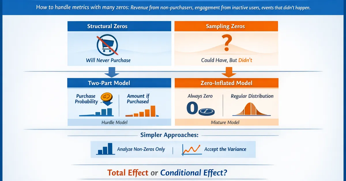
How to handle metrics with many zeros—revenue from non-purchasers, engagement from inactive users, events that didn't happen. Learn when to use zero-inflated models, two-part models, and simpler alternatives.
Quick Hits
- •Two populations: structural zeros (will never purchase) vs. sampling zeros (could but didn't)
- •Two-part models: separate probability of any value from amount given positive
- •Zero-inflated models: mixture of always-zero and standard distribution
- •Often simpler approaches work: analyze non-zeros separately, or just accept the variance
- •Choice depends on whether you care about total effect or conditional effect
TL;DR
Many product metrics have lots of zeros: revenue (non-purchasers), engagement (inactive users), support tickets (no issues). Standard methods struggle because zeros represent a distinct population, not just small values. Two-part models split the problem: model probability of any positive value, then model the amount given positive. Zero-inflated models treat some zeros as "structural" (will never be positive) and others as "sampling" (could be positive but weren't). Often, simpler approaches work: analyze positives separately, or use robust methods that handle the variance.
Why Zeros Are Different
Two Types of Zeros
Structural zeros: User fundamentally won't have this behavior
- Free users who can't purchase (paywall)
- Users in regions without the feature
- Bot accounts (no real engagement)
Sampling zeros: User could have the behavior but didn't in this period
- Purchaser who didn't buy this week
- Active user who didn't engage today
- Customer who had no support issues
Why This Matters
Standard models (linear regression, t-tests) treat all zeros the same—as small values. But:
- Structural zeros shouldn't be "converted" by treatment
- Combining populations inflates variance
- Mean is pulled toward zero, masking effects among actives
The Math Problem
For revenue with 80% zeros:
- Mean = 0.2 × (mean among buyers)
- Variance is huge (zero vs. non-zero dominates)
- Standard error is enormous → low power
Approaches to Zero-Heavy Data
Approach 1: Analyze Separately
Split into two analyses:
- Conversion: Did they have any positive value? (logistic regression)
- Amount: Among positives, what was the value? (standard methods)
import numpy as np
import pandas as pd
from scipy import stats
import statsmodels.api as sm


def separate_analysis(data, value_col, group_col):
    """
    Analyze zeros and positives separately.
    """
    results = {}

    # Part 1: Conversion (any positive value)
    data['is_positive'] = (data[value_col] > 0).astype(int)

    groups = sorted(data[group_col].unique())
    conv_control = data.loc[data[group_col] == groups[0], 'is_positive']
    conv_treatment = data.loc[data[group_col] == groups[1], 'is_positive']

    # Z-test for proportions
    n_c, n_t = len(conv_control), len(conv_treatment)
    p_c, p_t = conv_control.mean(), conv_treatment.mean()

    p_pooled = (conv_control.sum() + conv_treatment.sum()) / (n_c + n_t)
    se = np.sqrt(p_pooled * (1 - p_pooled) * (1/n_c + 1/n_t))
    z_stat = (p_t - p_c) / se
    p_value_conv = 2 * (1 - stats.norm.cdf(abs(z_stat)))

    results['conversion'] = {
        'control_rate': p_c,
        'treatment_rate': p_t,
        'lift': (p_t - p_c) / p_c if p_c > 0 else np.inf,
        'p_value': p_value_conv
    }

    # Part 2: Amount among positives
    pos_control = data.loc[(data[group_col] == groups[0]) & (data[value_col] > 0), value_col]
    pos_treatment = data.loc[(data[group_col] == groups[1]) & (data[value_col] > 0), value_col]

    if len(pos_control) > 1 and len(pos_treatment) > 1:
        t_stat, p_value_amount = stats.ttest_ind(pos_control, pos_treatment)

        results['amount_given_positive'] = {
            'control_mean': pos_control.mean(),
            'treatment_mean': pos_treatment.mean(),
            'lift': (pos_treatment.mean() - pos_control.mean()) / pos_control.mean(),
            'p_value': p_value_amount
        }

    # Combined effect (for context)
    all_control = data.loc[data[group_col] == groups[0], value_col]
    all_treatment = data.loc[data[group_col] == groups[1], value_col]

    results['overall'] = {
        'control_mean': all_control.mean(),
        'treatment_mean': all_treatment.mean(),
        'lift': (all_treatment.mean() - all_control.mean()) / all_control.mean() if all_control.mean() > 0 else np.inf
    }

    return results


# Example
np.random.seed(42)
n = 5000

# Simulate revenue data
data = pd.DataFrame({
    'group': np.random.choice(['control', 'treatment'], n),
    'revenue': np.where(
        np.random.binomial(1, 0.2, n),  # 20% purchasers
        np.random.lognormal(3, 1, n),    # Revenue among purchasers
        0
    )
})

# Treatment increases conversion slightly
treatment_mask = data['group'] == 'treatment'
data.loc[treatment_mask, 'revenue'] = np.where(
    np.random.binomial(1, 0.22, treatment_mask.sum()),  # 22% conversion
    np.random.lognormal(3, 1, treatment_mask.sum()),
    0
)

results = separate_analysis(data, 'revenue', 'group')

print("Separate Analysis Results")
print("=" * 50)
print(f"\nConversion (any purchase):")
print(f"  Control: {results['conversion']['control_rate']:.1%}")
print(f"  Treatment: {results['conversion']['treatment_rate']:.1%}")
print(f"  Lift: {results['conversion']['lift']:.1%}")
print(f"  p-value: {results['conversion']['p_value']:.4f}")

if 'amount_given_positive' in results:
    print(f"\nAmount (among purchasers):")
    print(f"  Control: ${results['amount_given_positive']['control_mean']:.2f}")
    print(f"  Treatment: ${results['amount_given_positive']['treatment_mean']:.2f}")
    print(f"  Lift: {results['amount_given_positive']['lift']:.1%}")
    print(f"  p-value: {results['amount_given_positive']['p_value']:.4f}")

print(f"\nOverall (all users):")
print(f"  Control: ${results['overall']['control_mean']:.2f}")
print(f"  Treatment: ${results['overall']['treatment_mean']:.2f}")
print(f"  Lift: {results['overall']['lift']:.1%}")
Approach 2: Two-Part (Hurdle) Model
Formally model both parts together:
1 - \pi & \text{if } y = 0 \\ \pi \cdot f(y | y > 0) & \text{if } y > 0 \end{cases}$$ Where $\pi$ is the probability of a positive value, and $f$ is the distribution of positive values. ```python import statsmodels.api as sm from scipy.optimize import minimize from scipy import stats class TwoPartModel: """ Two-part model: logistic for zero/positive, then log-normal for positives. """ def __init__(self): self.logit_model = None self.continuous_model = None def fit(self, X, y): """ Fit two-part model. Parameters: ----------- X : array-like Covariates (should include constant) y : array-like Response variable with zeros """ X = np.asarray(X) y = np.asarray(y) # Part 1: Logistic for any positive y_binary = (y > 0).astype(int) self.logit_model = sm.Logit(y_binary, X).fit(disp=0) # Part 2: OLS on log of positive values positive_mask = y > 0 if positive_mask.sum() > X.shape[1]: self.continuous_model = sm.OLS( np.log(y[positive_mask]), X[positive_mask] ).fit() return self def predict_probability(self, X): """Predict probability of positive value.""" return self.logit_model.predict(X) def predict_conditional_mean(self, X): """Predict mean given positive (on original scale).""" log_mean = self.continuous_model.predict(X) # Smearing adjustment for log-normal sigma = np.sqrt(self.continuous_model.mse_resid) return np.exp(log_mean + sigma**2 / 2) def predict_unconditional_mean(self, X): """Predict overall mean (including zeros).""" prob = self.predict_probability(X) conditional = self.predict_conditional_mean(X) return prob * conditional def summary(self): """Print model summaries.""" print("Part 1: Logistic (Probability of Positive)") print("=" * 50) print(self.logit_model.summary()) print("\n") print("Part 2: Log-Linear (Amount | Positive)") print("=" * 50) print(self.continuous_model.summary()) # Example: Treatment effect on revenue np.random.seed(42) n = 2000 # Generate data treatment = np.random.binomial(1, 0.5, n) # Treatment increases conversion probability prob_purchase = 0.15 + 0.05 * treatment purchased = np.random.binomial(1, prob_purchase) # Treatment also increases amount among purchasers log_revenue = 3 + 0.2 * treatment + np.random.normal(0, 1, n) revenue = np.where(purchased, np.exp(log_revenue), 0) # Fit two-part model X = sm.add_constant(treatment) model = TwoPartModel() model.fit(X, revenue) print("Two-Part Model Results") print("=" * 60) model.summary() # Treatment effects print("\n" + "=" * 60) print("Treatment Effects:") print("-" * 60) # On probability logit_coef = model.logit_model.params[1] logit_se = model.logit_model.bse[1] odds_ratio = np.exp(logit_coef) print(f"Probability of purchase:") print(f" Odds ratio: {odds_ratio:.3f}") print(f" 95% CI: ({np.exp(logit_coef - 1.96*logit_se):.3f}, {np.exp(logit_coef + 1.96*logit_se):.3f})") # On amount if model.continuous_model is not None: cont_coef = model.continuous_model.params[1] cont_se = model.continuous_model.bse[1] multiplier = np.exp(cont_coef) print(f"\nAmount given purchase:") print(f" Multiplier: {multiplier:.3f}") print(f" 95% CI: ({np.exp(cont_coef - 1.96*cont_se):.3f}, {np.exp(cont_coef + 1.96*cont_se):.3f})") # Predicted means X_control = np.array([[1, 0]]) X_treatment = np.array([[1, 1]]) mean_control = model.predict_unconditional_mean(X_control)[0] mean_treatment = model.predict_unconditional_mean(X_treatment)[0] print(f"\nPredicted overall revenue:") print(f" Control: ${mean_control:.2f}") print(f" Treatment: ${mean_treatment:.2f}") print(f" Lift: {(mean_treatment - mean_control) / mean_control:.1%}") ``` ### R Implementation ```r library(pscl) library(MASS) # Two-part model in R fit_two_part <- function(data, formula_binary, formula_continuous) { # Part 1: Logistic data$is_positive <- as.integer(data$revenue > 0) logit_model <- glm(is_positive ~ treatment, data = data, family = binomial) # Part 2: Log-linear among positives data_pos <- data[data$revenue > 0, ] lm_model <- lm(log(revenue) ~ treatment, data = data_pos) list( logit = logit_model, continuous = lm_model ) } # Zero-inflated models library(pscl) # Zero-inflated Poisson (for counts) zip_model <- zeroinfl(count ~ treatment | treatment, data = data, dist = "poisson") # Zero-inflated negative binomial zinb_model <- zeroinfl(count ~ treatment | treatment, data = data, dist = "negbin") summary(zinb_model) ``` --- ## Zero-Inflated Models ### The Mixture Concept Zero-inflated models assume data comes from a mixture: - With probability ψ: always zero (structural) - With probability 1-ψ: follows count distribution (may also produce zeros) $$P(Y = 0) = \psi + (1 - \psi) \cdot P(Y = 0 | \text{count model})$$ $$P(Y = k) = (1 - \psi) \cdot P(Y = k | \text{count model}), \quad k > 0$$ ### When to Use Zero-Inflated vs. Two-Part | Scenario | Model | Reasoning | |----------|-------|-----------| | Non-payers who could convert | Two-part | Zeros are "didn't buy yet" | | Mix of bots and real users | Zero-inflated | Some are fundamentally different | | Active users with no events | Either | Could go either way | | Structural ineligibility | Zero-inflated | Can't have positive value | ### Code: Zero-Inflated Poisson ```python from scipy.optimize import minimize from scipy.special import gammaln import numpy as np def fit_zip(y, X): """ Fit zero-inflated Poisson model. Parameters: ----------- y : array Count response X : array Covariates (with constant) for count model Returns dict with coefficients and standard errors. """ n = len(y) k = X.shape[1] def neg_log_likelihood(params): # Parameters: first k are Poisson coefficients, last 1 is logit(psi) beta = params[:k] logit_psi = params[k] psi = 1 / (1 + np.exp(-logit_psi)) # Probability of structural zero lambda_ = np.exp(X @ beta) # Log-likelihood ll = 0 for i in range(n): if y[i] == 0: # Zero can come from either component p_zero = psi + (1 - psi) * np.exp(-lambda_[i]) ll += np.log(p_zero + 1e-10) else: # Positive must come from Poisson ll += np.log(1 - psi + 1e-10) ll += y[i] * np.log(lambda_[i]) - lambda_[i] - gammaln(y[i] + 1) return -ll # Initial values init_params = np.zeros(k + 1) init_params[0] = np.log(y[y > 0].mean() + 0.1) # Intercept for Poisson init_params[k] = 0 # psi = 0.5 # Optimize result = minimize(neg_log_likelihood, init_params, method='BFGS') # Extract results beta = result.x[:k] psi = 1 / (1 + np.exp(-result.x[k])) return { 'poisson_coef': beta, 'psi': psi, 'converged': result.success, 'log_likelihood': -result.fun } # Example: Support ticket counts np.random.seed(42) n = 1000 treatment = np.random.binomial(1, 0.5, n) # 30% are structural zeros (never submit tickets) structural_zero = np.random.binomial(1, 0.3, n) # Among others, Poisson counts lambda_ = np.exp(0.5 - 0.3 * treatment) # Treatment reduces tickets counts = np.where( structural_zero, 0, np.random.poisson(lambda_) ) # Fit model X = np.column_stack([np.ones(n), treatment]) results = fit_zip(counts, X) print("Zero-Inflated Poisson Results") print("=" * 50) print(f"Structural zero probability (ψ): {results['psi']:.3f}") print(f"Poisson intercept: {results['poisson_coef'][0]:.3f}") print(f"Treatment effect on log-rate: {results['poisson_coef'][1]:.3f}") print(f"Rate ratio: {np.exp(results['poisson_coef'][1]):.3f}") ``` --- ## Comparing Approaches ### Simulation: Which Method Wins? ```python import numpy as np import pandas as pd from scipy import stats def simulate_zero_heavy(n_per_group, zero_rate, true_effect_conv, true_effect_amount): """ Simulate zero-heavy data with known treatment effects. """ # Control group is_positive_c = np.random.binomial(1, 1 - zero_rate, n_per_group) amount_c = np.where(is_positive_c, np.random.lognormal(3, 1, n_per_group), 0) # Treatment group is_positive_t = np.random.binomial(1, (1 - zero_rate) * (1 + true_effect_conv), n_per_group) amount_t = np.where( is_positive_t, np.random.lognormal(3 + np.log(1 + true_effect_amount), 1, n_per_group), 0 ) return amount_c, amount_t def compare_methods(n_simulations=500): """ Compare different methods for analyzing zero-heavy data. """ np.random.seed(42) results = { 'naive_ttest': [], 'log_ttest': [], # Log transform (excluding zeros) 'wilcoxon': [], 'separate_conv': [], 'separate_amount': [] } # True effects true_conv_effect = 0.10 # 10% lift in conversion true_amount_effect = 0.05 # 5% lift in amount among buyers for _ in range(n_simulations): control, treatment = simulate_zero_heavy( n_per_group=2000, zero_rate=0.8, # 80% zeros true_effect_conv=true_conv_effect, true_effect_amount=true_amount_effect ) # Method 1: Naive t-test _, p_naive = stats.ttest_ind(control, treatment) results['naive_ttest'].append(p_naive < 0.05) # Method 2: T-test on log (excluding zeros) log_c = np.log(control[control > 0]) log_t = np.log(treatment[treatment > 0]) _, p_log = stats.ttest_ind(log_c, log_t) results['log_ttest'].append(p_log < 0.05) # Method 3: Mann-Whitney _, p_mw = stats.mannwhitneyu(control, treatment, alternative='two-sided') results['wilcoxon'].append(p_mw < 0.05) # Method 4: Separate - conversion conv_c = (control > 0).mean() conv_t = (treatment > 0).mean() n = len(control) p_pool = (conv_c + conv_t) / 2 se = np.sqrt(p_pool * (1 - p_pool) * 2 / n) z = (conv_t - conv_c) / se results['separate_conv'].append(abs(z) > 1.96) # Method 5: Separate - amount among positives _, p_amount = stats.ttest_ind(control[control > 0], treatment[treatment > 0]) results['separate_amount'].append(p_amount < 0.05) # Power summary power_df = pd.DataFrame({ 'Method': ['Naive t-test', 'Log t-test (positives)', 'Mann-Whitney', 'Conversion test', 'Amount test (positives)'], 'Power': [np.mean(results['naive_ttest']), np.mean(results['log_ttest']), np.mean(results['wilcoxon']), np.mean(results['separate_conv']), np.mean(results['separate_amount'])] }) return power_df power_results = compare_methods() print("Power Comparison (500 simulations)") print("True effects: +10% conversion, +5% amount among buyers") print("Data: 80% zeros, n=2000 per group") print("=" * 50) print(power_results.to_string(index=False)) ``` ### Results Interpretation Typical findings: - **Naive t-test**: Low power (variance dominated by zeros) - **Log t-test**: Good power for amount effect, misses conversion effect - **Mann-Whitney**: Moderate power, tests stochastic dominance - **Conversion test**: High power for conversion effect - **Amount test**: High power for amount effect **Key insight**: Separate analyses have higher power for their respective effects. --- ## Decision Framework ``` START: Metric has many zeros ↓ QUESTION: What's your primary question? ├── Total effect (including zeros) → Continue └── Effect among actives only → Analyze non-zeros directly ↓ QUESTION: Are zeros structural or sampling? ├── Structural (will never be positive) → Zero-inflated model ├── Sampling (could be positive) → Two-part/hurdle model └── Unknown/Mixed → Two-part is usually safer ↓ QUESTION: How complex do you need? ├── Just want p-value → Separate analyses ├── Want combined inference → Formal two-part model └── Want predictions → Full model with covariates ↓ VALIDATE: Check model fit - Compare predicted vs. observed zero rate - Check distribution of positive predictions - Assess residuals in continuous part ``` --- ## Practical Recommendations ### When Simple Works 1. **Low stakes, directional answer**: Just compare means (accept variance) 2. **Clear separation**: Analyze conversion and amount separately 3. **Only one part matters**: Just test that part ### When to Model 1. **Need combined confidence interval**: Two-part model 2. **Covariates differ for zero vs. positive**: Separate covariate effects 3. **Structural zeros identifiable**: Zero-inflated model 4. **Prediction is goal**: Full model specification ### Reporting Always disclose: 1. What proportion of data are zeros 2. Which model/approach you used and why 3. Results for both parts if applicable 4. Sensitivity to modeling choices --- ## Related Methods - [Metric Distributions (Pillar)](/metric-distributions-product-analytics-heavy-tails-skew) - Full distributions overview - [Why Revenue Is Hard](/why-revenue-hard-log-normal-heavy-tails) - Heavy tails and whales - [Poisson vs. Negative Binomial](/poisson-vs-negative-binomial-modeling-counts-rates) - Count models - [Logistic Regression](/logistic-regression-conversion-interpretation-pitfalls) - Binary outcome modeling --- ## Key Takeaway Zeros in product metrics often represent distinct populations—users who won't engage vs. users who could but didn't. Standard methods that treat zeros as "small values" lose power and can mislead. Two-part models separate the "if" from the "how much," giving you targeted effects for each. Zero-inflated models explicitly handle structural zeros. But don't overcomplicate: often analyzing conversion and amount separately answers your question more directly than a fancy model. Choose based on what effect you're trying to measure and communicate. ---References
- https://doi.org/10.1177/0962280212443324
- https://doi.org/10.1002/sim.1401
- https://pubs.aeaweb.org/doi/10.1257/jep.15.4.157
- Mullahy, J. (1998). Much ado about two: reconsidering retransformation and the two-part model in health econometrics. *Journal of Health Economics*, 17(3), 247-281.
- Lambert, D. (1992). Zero-inflated Poisson regression, with an application to defects in manufacturing. *Technometrics*, 34(1), 1-14.
- Duan, N., Manning, W. G., Morris, C. N., & Newhouse, J. P. (1983). A comparison of alternative models for the demand for medical care. *Journal of Business & Economic Statistics*, 1(2), 115-126.
Frequently Asked Questions
When should I use a two-part model vs. zero-inflated model?
Can I just analyze non-zero values separately?
How many zeros is 'too many' for standard methods?
Key Takeaway
Zeros in product metrics often represent two distinct populations: users who will never engage (structural zeros) and users who could engage but didn't in this period (sampling zeros). Two-part models handle this by separately modeling if and how much. Zero-inflated models explicitly model the mixture. But simpler approaches—analyzing non-zeros separately or accepting higher variance—often suffice. Choose based on your business question: total effect or conditional effect.