Contents
Normality Tests Are Overrated: Better Diagnostics and Thresholds
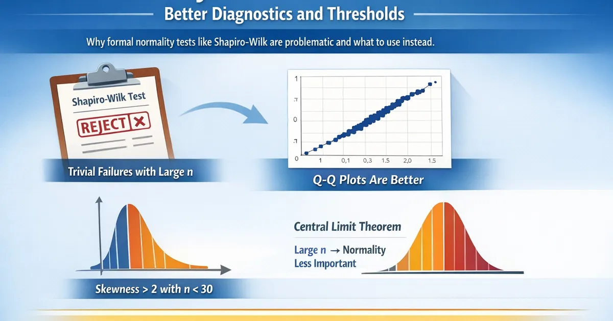
Why formal normality tests like Shapiro-Wilk are problematic and what to use instead. Learn practical thresholds for when non-normality actually matters.
Quick Hits
- •Normality tests reject trivial deviations with large n and miss important ones with small n
- •Q-Q plots are more informative than any formal test
- •Skewness > 2 with n < 30 is when you should worry
- •The Central Limit Theorem makes normality less critical for means
TL;DR
Formal normality tests like Shapiro-Wilk are problematic: with small samples they can't detect violations, with large samples they reject trivial deviations. Q-Q plots and skewness values provide more useful information. The key insight: normality of data matters less than you think because the Central Limit Theorem ensures the sampling distribution of means becomes normal with sufficient sample size.
The Problem with Normality Tests
The Paradox
import numpy as np
from scipy import stats
import matplotlib.pyplot as plt

def demonstrate_normality_test_paradox():
    """
    Show that normality tests fail exactly when we need them.
    """
    np.random.seed(42)
    n_sims = 1000

    # Test exponential data (clearly non-normal)
    sample_sizes = [10, 20, 30, 50, 100, 500, 1000]
    results = []

    for n in sample_sizes:
        rejections = 0
        for _ in range(n_sims):
            sample = np.random.exponential(10, n)
            _, p = stats.shapiro(sample) if n <= 5000 else stats.normaltest(sample)
            if p < 0.05:
                rejections += 1

        results.append({
            'n': n,
            'power': rejections / n_sims,
            'clt_applies': n >= 30
        })

    print("Shapiro-Wilk power to detect exponential (clearly non-normal):")
    print("-" * 50)
    for r in results:
        clt_note = " (CLT helps here)" if r['clt_applies'] else " (CLT weak)"
        print(f"n = {r['n']:4d}: {r['power']:5.1%} rejection rate{clt_note}")

    print("\nThe paradox:")
    print("- Small n: Low power to detect non-normality")
    print("- Large n: High power, but CLT makes normality less critical")


demonstrate_normality_test_paradox()
Real-World Impact
def test_trivial_deviations():
    """
    Show that large samples reject near-normal data.
    """
    np.random.seed(42)
    n_sims = 1000

    # Almost perfectly normal (just slightly skewed)
    results = []
    for n in [50, 100, 500, 1000, 5000]:
        rejections = 0
        for _ in range(n_sims):
            # Generate nearly normal data with tiny skew
            sample = stats.skewnorm.rvs(a=0.5, size=n)  # Very mild skew
            _, p = stats.shapiro(sample) if n <= 5000 else stats.normaltest(sample)
            if p < 0.05:
                rejections += 1
        results.append({'n': n, 'rejection_rate': rejections / n_sims})

    print("Rejection rate for NEARLY normal data (skew = 0.5):")
    print("(These rejections are statistically 'correct' but practically meaningless)")
    print("-" * 50)
    for r in results:
        print(f"n = {r['n']:4d}: {r['rejection_rate']:5.1%}")


test_trivial_deviations()
Q-Q Plots: The Better Diagnostic
How to Read a Q-Q Plot
from scipy.stats import probplot

def create_qq_examples():
    """
    Show Q-Q plots for different distributions.
    """
    np.random.seed(42)
    n = 100

    distributions = {
        'Normal': np.random.normal(0, 1, n),
        'Right-skewed': np.random.exponential(1, n),
        'Left-skewed': -np.random.exponential(1, n),
        'Heavy-tailed': np.random.standard_t(3, n),
        'Light-tailed': np.random.uniform(-2, 2, n),
        'Outliers': np.concatenate([np.random.normal(0, 1, n-3), [5, 6, -5]])
    }

    fig, axes = plt.subplots(2, 3, figsize=(15, 10))
    axes = axes.flatten()

    for ax, (name, data) in zip(axes, distributions.items()):
        probplot(data, dist="norm", plot=ax)
        ax.set_title(f'{name}\nSkew: {stats.skew(data):.2f}, Kurt: {stats.kurtosis(data):.2f}')
        ax.get_lines()[1].set_color('red')
        ax.get_lines()[1].set_linewidth(2)

    plt.tight_layout()
    return fig


def interpret_qq_pattern(data):
    """
    Interpret Q-Q plot patterns programmatically.
    """
    # Generate theoretical quantiles
    n = len(data)
    theoretical = stats.norm.ppf((np.arange(1, n + 1) - 0.5) / n)
    empirical = np.sort(data)

    # Calculate deviations
    residuals = empirical - (theoretical * np.std(data) + np.mean(data))

    # Check for patterns
    interpretation = []

    # Right skew: positive residuals at high end
    if np.mean(residuals[int(0.9*n):]) > 0.5 * np.std(data):
        interpretation.append("Right-skewed (upper tail extends too far)")

    # Left skew: negative residuals at low end
    if np.mean(residuals[:int(0.1*n)]) < -0.5 * np.std(data):
        interpretation.append("Left-skewed (lower tail extends too far)")

    # Heavy tails: both extremes deviate
    if (np.mean(residuals[int(0.9*n):]) > 0.3 * np.std(data) and
        np.mean(residuals[:int(0.1*n)]) < -0.3 * np.std(data)):
        interpretation.append("Heavy-tailed (both extremes deviate)")

    # Outliers: isolated extreme points
    z_scores = np.abs(stats.zscore(data))
    if np.sum(z_scores > 3) > 0:
        interpretation.append(f"Outliers detected: {np.sum(z_scores > 3)} points > 3 SD")

    if not interpretation:
        interpretation.append("Reasonably normal")

    return interpretation
Practical Q-Q Guidelines
| Pattern | What It Means | Concern Level |
|---|---|---|
| Points on line | Normal | None |
| S-curve (up-down) | Skewed | Moderate |
| Both ends above line | Heavy tails | Moderate-High |
| Both ends below line | Light tails | Low |
| Few isolated points off | Outliers | Investigate |
Practical Thresholds
Skewness Guidelines
def skewness_guidelines(data):
    """
    Practical guidance based on skewness and sample size.
    """
    n = len(data)
    skew = stats.skew(data)
    kurt = stats.kurtosis(data)  # Excess kurtosis

    assessment = {
        'n': n,
        'skewness': skew,
        'kurtosis': kurt,
        'interpretation': []
    }

    # Skewness assessment
    if abs(skew) < 0.5:
        assessment['skewness_level'] = 'Minimal'
    elif abs(skew) < 1:
        assessment['skewness_level'] = 'Moderate'
    elif abs(skew) < 2:
        assessment['skewness_level'] = 'Substantial'
    else:
        assessment['skewness_level'] = 'Severe'

    # Recommendation based on n and skewness
    if n >= 100:
        if abs(skew) < 2:
            assessment['recommendation'] = 'Standard methods OK (CLT applies)'
        else:
            assessment['recommendation'] = 'Consider robust methods despite large n'
    elif n >= 30:
        if abs(skew) < 1:
            assessment['recommendation'] = 'Standard methods likely OK'
        elif abs(skew) < 2:
            assessment['recommendation'] = 'Borderline—consider robust methods'
        else:
            assessment['recommendation'] = 'Use robust methods'
    else:  # n < 30
        if abs(skew) < 0.5:
            assessment['recommendation'] = 'Standard methods cautiously OK'
        else:
            assessment['recommendation'] = 'Use robust methods or exact tests'

    return assessment


# Examples
test_cases = [
    np.random.normal(100, 15, 200),  # Normal, large n
    np.random.exponential(20, 15),    # Skewed, small n
    np.random.exponential(20, 100),   # Skewed, large n
]

for i, data in enumerate(test_cases):
    result = skewness_guidelines(data)
    print(f"\nCase {i+1}:")
    print(f"  n = {result['n']}, skewness = {result['skewness']:.2f}")
    print(f"  Level: {result['skewness_level']}")
    print(f"  Recommendation: {result['recommendation']}")
Decision Table
| Sample Size | Skewness | Recommendation |
|---|---|---|
| n < 15 | Any | Use exact tests or bootstrap |
| n = 15-30 | |skew| < 0.5 | Standard methods cautiously OK |
| n = 15-30 | |skew| 0.5-2 | Consider robust methods |
| n = 15-30 | |skew| > 2 | Use robust methods |
| n = 30-100 | |skew| < 1 | Standard methods OK |
| n = 30-100 | |skew| > 1 | Consider robust methods |
| n > 100 | |skew| < 2 | Standard methods OK (CLT) |
| n > 100 | |skew| > 2 | Consider robust despite CLT |
What Actually Matters
Normality of What?
| Test | Formal requirement | Practical reality | Implication |
|---|---|---|---|
| t-test | Populations are normally distributed | Sampling distribution of mean is normal | CLT saves you with large n |
| ANOVA | Residuals are normally distributed | Sampling distribution of group means | Same as t-test — CLT helps |
| Regression | Residuals are normally distributed | Affects CI and hypothesis tests, not coefficients | Coefficients are unbiased either way |
| Prediction intervals | Need distributional assumption | Actually need normality here | Use quantile regression if violated |
The CLT in Action
def visualize_clt_rescue():
    """
    Show how CLT makes normality less critical.
    """
    np.random.seed(42)

    # Very non-normal population (bimodal)
    def bimodal_sample(n):
        return np.concatenate([
            np.random.normal(-3, 1, n // 2),
            np.random.normal(3, 1, n - n // 2)
        ])

    sample_sizes = [5, 10, 30, 100]
    n_simulations = 10000

    fig, axes = plt.subplots(1, 4, figsize=(16, 4))

    for ax, n in zip(axes, sample_sizes):
        # Simulate sampling distribution of mean
        means = [bimodal_sample(n).mean() for _ in range(n_simulations)]

        ax.hist(means, bins=50, density=True, alpha=0.7, label='Sample means')

        # Overlay normal
        x = np.linspace(min(means), max(means), 100)
        ax.plot(x, stats.norm.pdf(x, np.mean(means), np.std(means)),
                'r-', linewidth=2, label='Normal fit')

        # Shapiro-Wilk on first 5000
        _, p = stats.shapiro(means[:5000])
        ax.set_title(f'n = {n}\nShapiro p = {p:.4f}')
        ax.set_xlabel('Sample Mean')

    axes[0].set_ylabel('Density')
    plt.suptitle('CLT: Sample means become normal even from bimodal population', y=1.02)
    plt.tight_layout()
    return fig
Better Diagnostic Workflow
def normality_diagnostic_workflow(data, alpha=0.05):
    """
    Complete normality assessment without over-relying on tests.
    """
    n = len(data)
    skew = stats.skew(data)
    kurt = stats.kurtosis(data)

    print("NORMALITY DIAGNOSTIC REPORT")
    print("=" * 50)

    # 1. Basic stats
    print(f"\nSample size: {n}")
    print(f"Skewness: {skew:.3f}")
    print(f"Excess kurtosis: {kurt:.3f}")

    # 2. Visual assessment guidance
    print("\nVISUAL ASSESSMENT:")
    print("-" * 30)
    print("(Examine Q-Q plot)")

    if abs(skew) < 0.5 and abs(kurt) < 1:
        print("Expected: Points should follow the line closely")
    elif abs(skew) > 1:
        direction = "right" if skew > 0 else "left"
        print(f"Expected: S-curve indicating {direction} skew")
    if kurt > 3:
        print("Expected: Points above line at both extremes (heavy tails)")

    # 3. Formal test (with caveats)
    print("\nFORMAL TEST (interpret cautiously):")
    print("-" * 30)
    if n <= 5000:
        stat, p = stats.shapiro(data)
        print(f"Shapiro-Wilk: W = {stat:.4f}, p = {p:.4f}")
    else:
        stat, p = stats.normaltest(data)
        print(f"D'Agostino-Pearson: stat = {stat:.4f}, p = {p:.4f}")

    if n > 100 and p < 0.05:
        print("⚠️  With n > 100, test may reject trivial deviations")
    if n < 30 and p > 0.05:
        print("⚠️  With n < 30, test may miss important violations")

    # 4. Practical recommendation
    print("\nRECOMMENDATION:")
    print("-" * 30)

    if n >= 50 and abs(skew) < 2:
        print("✓ Standard methods should be fine (CLT applies)")
    elif n >= 30 and abs(skew) < 1:
        print("✓ Standard methods likely OK")
    elif abs(skew) > 2 or (n < 30 and abs(skew) > 0.5):
        print("⚠️  Consider robust methods:")
        print("   - Bootstrap confidence intervals")
        print("   - Rank-based tests (Mann-Whitney, Wilcoxon)")
        print("   - Trimmed means")
    else:
        print("Standard methods are probably fine, but:")
        print("   - Welch's t-test is a safe default")
        print("   - Bootstrap provides robustness")

    return {'skewness': skew, 'kurtosis': kurt, 'n': n, 'p_value': p}


# Example
np.random.seed(42)
skewed_data = np.random.exponential(10, 35)
normality_diagnostic_workflow(skewed_data)
R Implementation
library(moments)

normality_diagnostic <- function(data) {
  n <- length(data)
  skew <- skewness(data)
  kurt <- kurtosis(data) - 3  # Excess kurtosis

  cat("NORMALITY DIAGNOSTIC\n")
  cat(rep("=", 40), "\n\n")

  cat(sprintf("n = %d\n", n))
  cat(sprintf("Skewness = %.3f\n", skew))
  cat(sprintf("Excess Kurtosis = %.3f\n\n", kurt))

  # Shapiro-Wilk
  if (n >= 3 && n <= 5000) {
    sw <- shapiro.test(data)
    cat(sprintf("Shapiro-Wilk: W = %.4f, p = %.4f\n\n", sw$statistic, sw$p.value))
  }

  # Q-Q plot
  par(mfrow = c(1, 2))
  hist(data, main = "Histogram", probability = TRUE)
  curve(dnorm(x, mean(data), sd(data)), add = TRUE, col = "red", lwd = 2)
  qqnorm(data, main = "Q-Q Plot")
  qqline(data, col = "red", lwd = 2)
  par(mfrow = c(1, 1))

  # Recommendation
  cat("RECOMMENDATION:\n")
  cat(rep("-", 30), "\n")

  if (n >= 50 && abs(skew) < 2) {
    cat("Standard methods should be fine (CLT applies)\n")
  } else if (abs(skew) > 2 || (n < 30 && abs(skew) > 0.5)) {
    cat("Consider robust methods or transformations\n")
  } else {
    cat("Standard methods likely OK, Welch is safe default\n")
  }
}

# Usage
# data <- rexp(50, 0.1)
# normality_diagnostic(data)
Related Methods
- Assumption Checks Master Guide — The pillar article
- Transformations Guide — When transformations help
- Robust Statistics Toolbox — Methods that don't need normality
- Visual Diagnostics — Diagnostic plots for assumptions
Key Takeaway
Normality tests have a fundamental flaw: they're underpowered when sample size is small (when normality matters most) and overpowered when sample size is large (when CLT makes normality less critical). Use Q-Q plots and skewness thresholds instead. With skewness under 2 and sample sizes over 30, standard methods usually work fine. When in doubt, robust methods rarely hurt.
References
- https://www.jstor.org/stable/2685122
- https://www.jstor.org/stable/1165059
- Rochon, J., Gondan, M., & Kieser, M. (2012). To test or not to test: Preliminary assessment of normality when comparing two independent samples. *BMC Medical Research Methodology*, 12(1), 81.
- Razali, N. M., & Wah, Y. B. (2011). Power comparisons of Shapiro-Wilk, Kolmogorov-Smirnov, Lilliefors and Anderson-Darling tests. *Journal of Statistical Modeling and Analytics*, 2(1), 21-33.
- Lumley, T., Diehr, P., Emerson, S., & Chen, L. (2002). The importance of the normality assumption in large public health data sets. *Annual Review of Public Health*, 23(1), 151-169.
Frequently Asked Questions
Should I run Shapiro-Wilk before every t-test?
What makes a Q-Q plot 'bad enough' to worry?
At what sample size does normality stop mattering?
Key Takeaway
Normality tests have a fundamental problem: they're underpowered when sample size is small (when normality matters most) and overpowered when sample size is large (when it matters least due to CLT). Use Q-Q plots, skewness thresholds, and sample size considerations instead.