Contents
Multiple Comparisons: When Bonferroni Is Too Conservative
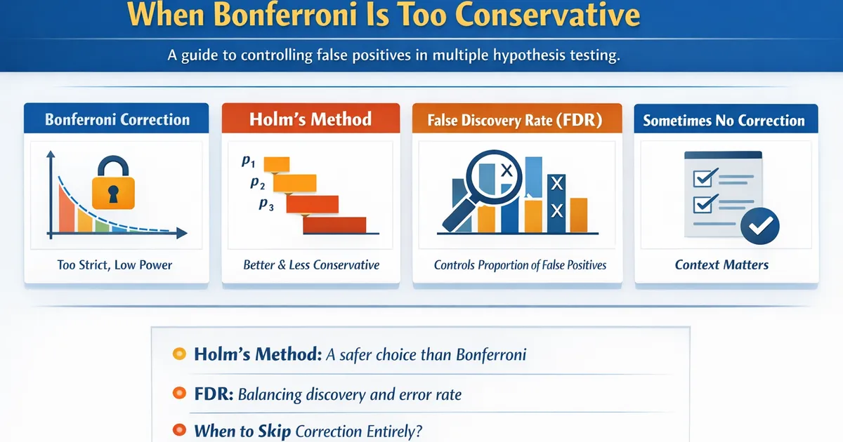
A practical guide to controlling false positives when testing multiple hypotheses. Learn when Bonferroni over-corrects and better alternatives like Holm, FDR, and when to skip correction entirely.
Quick Hits
- •Bonferroni is simple but often too conservative, reducing power substantially
- •Holm's method is always as good or better than Bonferroni—no reason not to use it
- •FDR controls proportion of false positives among discoveries, not overall error rate
- •Not every multiple test situation requires correction
TL;DR
Testing multiple hypotheses inflates false positive rates—with 20 tests at , you expect one false positive by chance. Bonferroni correction () controls this but is often too conservative, slashing power. Better alternatives: Holm's step-down method (always preferred over Bonferroni), FDR for exploratory work, or no correction when tests are truly independent decisions.
The Multiple Comparisons Problem
Why It Matters
import numpy as np
from scipy import stats
import pandas as pd

def demonstrate_multiple_testing_problem():
    """
    Show how multiple testing inflates false positive rate.
    """
    np.random.seed(42)

    # Simulate 20 tests, all null (no real effects)
    n_tests = 20
    n_sims = 10000
    alpha = 0.05

    any_false_positive = 0

    for _ in range(n_sims):
        p_values = []
        for _ in range(n_tests):
            # Two groups with same mean (null is true)
            g1 = np.random.normal(0, 1, 30)
            g2 = np.random.normal(0, 1, 30)
            _, p = stats.ttest_ind(g1, g2)
            p_values.append(p)

        # Any significant?
        if min(p_values) < alpha:
            any_false_positive += 1

    familywise_error = any_false_positive / n_sims
    expected = 1 - (1 - alpha)**n_tests

    print("Multiple Testing Without Correction:")
    print("-" * 50)
    print(f"Number of tests: {n_tests}")
    print(f"Alpha per test: {alpha}")
    print(f"Expected FWER: {expected:.3f}")
    print(f"Observed FWER: {familywise_error:.3f}")
    print()
    print(f"You have a {familywise_error:.0%} chance of at least one")
    print(f"false positive, even when ALL nulls are true!")


demonstrate_multiple_testing_problem()
The Math
Probability of at least one false positive:
For tests at :
Correction Methods
Bonferroni
The simplest approach: divide by the number of tests.
def bonferroni_correction(p_values, alpha=0.05):
    """
    Bonferroni correction: reject if p < alpha/k.
    """
    k = len(p_values)
    adjusted_alpha = alpha / k

    results = []
    for i, p in enumerate(p_values):
        results.append({
            'test': i + 1,
            'p_value': p,
            'adjusted_p': min(p * k, 1.0),  # Adjusted p-value
            'significant': p < adjusted_alpha
        })

    return pd.DataFrame(results), adjusted_alpha


# Example
np.random.seed(42)
p_values = [0.001, 0.01, 0.02, 0.04, 0.06, 0.10, 0.15, 0.30, 0.50, 0.90]

df, adj_alpha = bonferroni_correction(p_values)
print("Bonferroni Correction:")
print("-" * 50)
print(f"Original α: 0.05")
print(f"Adjusted α: {adj_alpha:.4f}")
print()
print(df.to_string(index=False))
Why Bonferroni Is Too Conservative
def demonstrate_bonferroni_conservatism():
    """
    Show how Bonferroni reduces power dramatically.
    """
    np.random.seed(42)
    n_sims = 5000

    # 10 tests, 3 have real effects
    n_tests = 10
    true_effects = [0.5, 0.5, 0.5, 0, 0, 0, 0, 0, 0, 0]  # First 3 are real

    # Track power for each method
    results = {'Uncorrected': [], 'Bonferroni': [], 'Holm': [], 'FDR': []}

    for _ in range(n_sims):
        p_values = []
        for effect in true_effects:
            g1 = np.random.normal(0, 1, 50)
            g2 = np.random.normal(effect, 1, 50)
            _, p = stats.ttest_ind(g1, g2)
            p_values.append(p)

        p_values = np.array(p_values)

        # Uncorrected: just count p < 0.05 for true effects
        results['Uncorrected'].append(np.sum(p_values[:3] < 0.05))

        # Bonferroni
        results['Bonferroni'].append(np.sum(p_values[:3] < 0.05/n_tests))

        # Holm (we'll implement below)
        holm_sig = holm_correction(p_values, 0.05)
        results['Holm'].append(np.sum(holm_sig[:3]))

        # BH-FDR
        fdr_sig = benjamini_hochberg(p_values, 0.05)
        results['FDR'].append(np.sum(fdr_sig[:3]))

    # Average power per true effect
    print("Power Comparison (3 true effects out of 10 tests):")
    print("-" * 50)
    for method, detections in results.items():
        avg_power = np.mean(detections) / 3  # Divide by number of true effects
        print(f"{method:<15}: {avg_power:.1%} average power per true effect")


def holm_correction(p_values, alpha=0.05):
    """
    Holm's step-down correction.
    """
    n = len(p_values)
    sorted_idx = np.argsort(p_values)
    sorted_p = p_values[sorted_idx]

    significant = np.zeros(n, dtype=bool)

    for i, (idx, p) in enumerate(zip(sorted_idx, sorted_p)):
        if p < alpha / (n - i):
            significant[idx] = True
        else:
            break  # Stop at first non-significant

    return significant


def benjamini_hochberg(p_values, alpha=0.05):
    """
    Benjamini-Hochberg FDR correction.
    """
    n = len(p_values)
    sorted_idx = np.argsort(p_values)
    sorted_p = p_values[sorted_idx]

    # Find largest k where p(k) <= k*alpha/n
    significant = np.zeros(n, dtype=bool)
    max_k = 0

    for k in range(n):
        if sorted_p[k] <= (k + 1) * alpha / n:
            max_k = k + 1

    # All up to max_k are significant
    for k in range(max_k):
        significant[sorted_idx[k]] = True

    return significant


demonstrate_bonferroni_conservatism()
Better Alternatives
Holm's Step-Down Method
Always at least as powerful as Bonferroni, never less conservative. No reason not to use it.
def holm_detailed(p_values, alpha=0.05):
    """
    Holm's method with step-by-step explanation.
    """
    n = len(p_values)
    sorted_idx = np.argsort(p_values)
    sorted_p = p_values[sorted_idx]

    print("Holm's Step-Down Procedure:")
    print("-" * 60)
    print(f"{'Step':<6} {'p-value':<12} {'Threshold':<12} {'Decision':<15}")
    print("-" * 60)

    significant = np.zeros(n, dtype=bool)
    all_rejected = True

    for i in range(n):
        threshold = alpha / (n - i)
        reject = sorted_p[i] < threshold and all_rejected

        if reject:
            significant[sorted_idx[i]] = True
            decision = "Reject"
        else:
            all_rejected = False
            decision = "Fail to reject"

        print(f"{i+1:<6} {sorted_p[i]:<12.4f} {threshold:<12.4f} {decision:<15}")

    print("-" * 60)
    print(f"Total rejected: {significant.sum()}")

    return significant


# Example
p_values = np.array([0.001, 0.008, 0.015, 0.025, 0.04, 0.06, 0.10])
holm_detailed(p_values)
False Discovery Rate (FDR)
FWER (Family-Wise Error Rate): Controls P(at least 1 false positive). Interpretation: "I'm 95% confident ALL discoveries are real." Use when each false positive is very costly. Methods: Bonferroni, Holm, Hochberg.
FDR (False Discovery Rate): Controls E[false positives / all positives]. Interpretation: "On average, 5% of my discoveries are false." Use when doing exploratory analysis and you'll follow up. Methods: Benjamini-Hochberg, Benjamini-Yekutieli.
For example, with 100 tests and 10 true effects: FWER = 0.05 means "I'm 95% sure I have NO false positives" (very strict, might miss real effects). FDR = 0.05 means "of my discoveries, ~5% are false positives" (if you find 15 significant, expect ~1 false).
def benjamini_hochberg_detailed(p_values, alpha=0.05):
    """
    BH-FDR procedure with explanation.
    """
    n = len(p_values)
    sorted_idx = np.argsort(p_values)
    sorted_p = p_values[sorted_idx]

    print("Benjamini-Hochberg FDR Procedure:")
    print("-" * 60)
    print(f"{'Rank':<6} {'p-value':<12} {'BH threshold':<15} {'Significant':<12}")
    print("-" * 60)

    # Find largest k where p(k) <= k*alpha/n
    max_k = 0
    for k in range(n):
        threshold = (k + 1) * alpha / n
        if sorted_p[k] <= threshold:
            max_k = k + 1

    for k in range(n):
        threshold = (k + 1) * alpha / n
        sig = "Yes" if k < max_k else "No"
        print(f"{k+1:<6} {sorted_p[k]:<12.4f} {threshold:<15.4f} {sig:<12}")

    print("-" * 60)
    print(f"Reject all with rank <= {max_k}")

    significant = np.zeros(n, dtype=bool)
    for k in range(max_k):
        significant[sorted_idx[k]] = True

    return significant


# Example
p_values = np.array([0.001, 0.005, 0.01, 0.02, 0.03, 0.04, 0.08, 0.15, 0.30, 0.60])
benjamini_hochberg_detailed(p_values)
Comparison of Methods
def compare_correction_methods(p_values, alpha=0.05):
    """
    Compare different correction methods side by side.
    """
    n = len(p_values)

    # Sort for display
    sorted_idx = np.argsort(p_values)
    sorted_p = p_values[sorted_idx]

    methods = {
        'Uncorrected': lambda p: p < alpha,
        'Bonferroni': lambda p: p < alpha/n,
        'Holm': lambda p: holm_correction(p, alpha),
        'BH-FDR': lambda p: benjamini_hochberg(p, alpha)
    }

    results = {}
    for name, method in methods.items():
        if name in ['Holm', 'BH-FDR']:
            results[name] = method(p_values)
        else:
            results[name] = np.array([method(p) for p in p_values])

    # Display
    print("Method Comparison:")
    print("=" * 70)
    print(f"{'p-value':<12}", end='')
    for name in methods:
        print(f"{name:<12}", end='')
    print()
    print("-" * 70)

    for i, (idx, p) in enumerate(zip(sorted_idx, sorted_p)):
        print(f"{p:<12.4f}", end='')
        for name in methods:
            sig = "Yes" if results[name][idx] else "No"
            print(f"{sig:<12}", end='')
        print()

    print("-" * 70)
    print(f"{'Total sig:':<12}", end='')
    for name in methods:
        print(f"{results[name].sum():<12}", end='')
    print()


# Example
np.random.seed(42)
p_values = np.array([0.001, 0.008, 0.012, 0.024, 0.035, 0.048, 0.06, 0.12, 0.25, 0.55])
compare_correction_methods(p_values)
When NOT to Correct
Independent Decisions
Independent decisions. Example: testing 3 different products for different markets. Each decision is separate; a false positive in one doesn't affect the others.
Planned comparisons. Example: treatment vs. control (planned), other comparisons exploratory. The primary hypothesis is a single test; don't penalize for exploratory tests.
Replication settings. Example: confirming a previous finding. Prior evidence reduces the false positive concern.
Descriptive analyses. Example: exploring patterns to generate hypotheses. You're not making claims, just describing data.
The Decision Framework
1. Are you testing multiple hypotheses? If no, no correction needed.
2. Are the tests related (answering one question)? If no (separate decisions), possibly no correction needed.
3. What's the cost of false positives?
- Very high (each false positive is costly) → Use FWER control (Holm preferred)
- Moderate (can follow up to verify) → Use FDR (Benjamini-Hochberg)
- Low (exploratory, just generating hypotheses) → Consider no correction; report all p-values
4. Which FWER method? Always use Holm over Bonferroni — same guarantee, more power.
5. Report transparently: Number of tests conducted, correction method used (and why), and both raw and adjusted p-values.
Common Scenarios
Scenario 1: Post-Hoc Pairwise Comparisons
The number of pairwise comparisons grows quickly: 4 groups = 6 comparisons, 5 groups = 10, 6 groups = 15.
Options:
- Tukey's HSD — Controls FWER, designed for this exact situation.
- Holm — General purpose, good choice.
- Dunnett's — If only comparing to a single control group (fewer comparisons, more power).
Note: if the ANOVA is not significant, post-hoc comparisons may not be needed.
Scenario 2: Multiple Outcomes
When testing an intervention on multiple outcomes (e.g., engagement, revenue, retention):
- Pre-specify a primary outcome. Only correct for secondary outcomes. The primary gets full alpha.
- Correct across all. Use Holm or FDR. More conservative for the primary outcome.
- Use a composite outcome. Combine outcomes into a single metric. Single test, no correction needed.
Scenario 3: Exploratory Analysis
This is common in data mining, genomics, and A/B test segmentation.
- Use FDR (Benjamini-Hochberg). Accepts ~5% false discoveries. Much more power than FWER methods.
- Report all p-values. Let readers assess. Show the distribution of p-values.
- Plan for validation. Exploratory findings need replication. Don't over-interpret significant results.
- Be transparent. Report the total number of tests and explain why you chose FDR vs. FWER.
R Implementation
# Multiple comparison corrections in R

p_values <- c(0.001, 0.008, 0.015, 0.025, 0.04, 0.06, 0.10)

# Built-in corrections
p.adjust(p_values, method = "bonferroni")
p.adjust(p_values, method = "holm")
p.adjust(p_values, method = "BH")  # Benjamini-Hochberg
p.adjust(p_values, method = "BY")  # Benjamini-Yekutieli

# Compare all methods
methods <- c("bonferroni", "holm", "hochberg", "BH", "BY")
adjusted <- sapply(methods, function(m) p.adjust(p_values, method = m))
colnames(adjusted) <- methods
print(adjusted)

# For post-hoc after ANOVA
library(emmeans)
model <- aov(value ~ group, data = df)
emmeans(model, pairwise ~ group, adjust = "tukey")
emmeans(model, pairwise ~ group, adjust = "holm")
Summary Table
| Method | Controls | Power | Best For |
|---|---|---|---|
| Bonferroni | FWER | Lowest | Simple, few tests |
| Holm | FWER | Good | General FWER control |
| Hochberg | FWER | Better | Independent tests |
| BH (FDR) | FDR | High | Exploratory, many tests |
| None | Nothing | Highest | Independent decisions |
Related Methods
- Assumption Checks Master Guide — The pillar article
- Post-Hoc Tests — Pairwise comparisons
- Multiple Experiments — A/B testing context
Key Takeaway
Multiple comparison correction is necessary when many related tests inflate false positive rates. However, Bonferroni is usually too conservative. Holm's method is strictly better and should be your default for FWER control. For exploratory work with many tests, FDR (Benjamini-Hochberg) provides a better power-protection tradeoff. And sometimes—when tests represent independent decisions—no correction is appropriate. Always report how many tests you ran and how you handled multiplicity.
References
- https://www.jstor.org/stable/4615733
- https://www.jstor.org/stable/2346101
- Hochberg, Y., & Benjamini, Y. (1990). More powerful procedures for multiple significance testing. *Statistics in Medicine*, 9(7), 811-818.
- Benjamini, Y., & Hochberg, Y. (1995). Controlling the false discovery rate: A practical and powerful approach to multiple testing. *Journal of the Royal Statistical Society: Series B*, 57(1), 289-300.
- Holm, S. (1979). A simple sequentially rejective multiple test procedure. *Scandinavian Journal of Statistics*, 6(2), 65-70.
Frequently Asked Questions
When should I correct for multiple comparisons?
Why is Bonferroni 'too conservative'?
What's the difference between FWER and FDR?
Key Takeaway
Multiple comparison correction is necessary when multiple related tests inflate false positive rates. However, Bonferroni is often too conservative. Holm's step-down method is always better and should be the default. For exploratory analyses with many tests, FDR provides a better power-protection tradeoff. Sometimes, no correction is appropriate—it depends on the decision context.