Contents
Logistic Regression for Conversion: Interpretation and Common Pitfalls
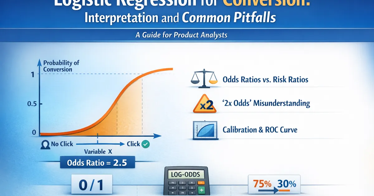
A practical guide to logistic regression for product analysts. Learn to interpret odds ratios correctly, avoid common mistakes, and communicate results to stakeholders who don't think in log-odds.
Quick Hits
- •Use logistic regression when your outcome is binary (converted/not, clicked/not)
- •Coefficients are in log-odds; exponentiate to get odds ratios
- •Odds ratios ≠ risk ratios - don't confuse them when outcomes are common
- •An odds ratio of 2 doesn't mean 'twice as likely' unless base rate is low
- •Check calibration, not just discrimination (AUC)
TL;DR
Logistic regression models binary outcomes (yes/no, converted/not, churned/retained) by predicting the log-odds of success. While technically straightforward, interpretation trips up many analysts. Odds ratios aren't intuitive, don't equal risk ratios when outcomes are common, and "twice the odds" doesn't mean "twice as likely." This guide shows you how to fit, interpret, and communicate logistic regression results correctly.
When to Use Logistic Regression
Use logistic regression when:
- Outcome is binary: Converted/not, clicked/not, churned/retained
- You want to understand predictors: Which factors affect conversion?
- You want to predict probability: What's the chance this user converts?
- You need to control for confounders: Effect of X on Y, adjusting for Z
Don't use when:
- Outcome is continuous → use linear regression
- Outcome is count → use Poisson/negative binomial
- Outcome has multiple categories → use multinomial logistic
The Logistic Model
The Equation
Where:
- = probability of the outcome (conversion)
- = odds
- = log-odds (or logit)
Solving for Probability
This is the sigmoid function, which squishes any linear combination to the 0-1 range.
Interpreting Coefficients
Raw Coefficients: Log-Odds
= change in log-odds for a one-unit increase in
Problem: Nobody thinks in log-odds.
Odds Ratios: Exponentiated Coefficients
= odds ratio (OR) for a one-unit increase in
Interpretation: "The odds of conversion are OR times higher/lower for each unit increase in "
Example
Model: log-odds(conversion) = -2.5 + 0.3(emails) - 0.8(price_tier)
| Variable | Coefficient | Odds Ratio | Interpretation |
|---|---|---|---|
| Intercept | -2.5 | 0.08 | Baseline odds |
| Emails | 0.3 | 1.35 | Each email increases odds by 35% |
| Price tier | -0.8 | 0.45 | Each tier increase cuts odds by 55% |
The Odds Ratio Trap
Odds Ratio Risk Ratio
When the outcome is common (>10%), odds ratios and risk ratios diverge significantly.
Example:
- Control group: 40% convert (odds = 0.67)
- Treatment group: 57% convert (odds = 1.33)
- Odds ratio: 1.33/0.67 = 2.0
- Risk ratio: 57%/40% = 1.43
Saying "twice the odds" when the probability only increased 43% is misleading.
The Rare Disease Assumption
Odds ratios approximate risk ratios only when:
- Base rate < 10%
- Outcome is "rare"
For common outcomes (like many conversion rates), this approximation fails.
What To Do
- Report odds ratios with clear language ("odds ratio", not "X times more likely")
- Calculate predicted probabilities for interpretable scenarios
- Use marginal effects for stakeholder communication
From Odds Ratios to Useful Numbers
Approach 1: Predicted Probabilities
Instead of OR=1.35, say: "Users who received 5 emails have a predicted conversion rate of 8.2%, compared to 6.1% for users who received no emails."
# Calculate predicted probabilities at specific values
import numpy as np

def predict_probability(intercept, coefficients, values):
    """Convert log-odds to probability."""
    log_odds = intercept + np.dot(coefficients, values)
    return 1 / (1 + np.exp(-log_odds))

# Model: log-odds = -2.5 + 0.3*emails - 0.8*price_tier
intercept = -2.5
coefficients = [0.3, -0.8]

# Compare: 0 emails vs 5 emails (price_tier=1)
p_0_emails = predict_probability(intercept, coefficients, [0, 1])
p_5_emails = predict_probability(intercept, coefficients, [5, 1])

print(f"0 emails: {p_0_emails:.1%}")
print(f"5 emails: {p_5_emails:.1%}")
print(f"Difference: {(p_5_emails - p_0_emails):.1%} percentage points")
Approach 2: Average Marginal Effects
The average marginal effect (AME) is the average change in probability for a one-unit change in X, across all observations.
import statsmodels.api as sm
import numpy as np

# After fitting model
# model = sm.Logit(y, X).fit()

# Average marginal effect
def average_marginal_effect(model, X, var_index):
    """Calculate AME for a continuous variable."""
    probs = model.predict(X)
    # Derivative of sigmoid at each point
    dydx = probs * (1 - probs) * model.params[var_index]
    return np.mean(dydx)
Approach 3: Scenario Comparison
Create a table showing predicted probabilities for meaningful scenarios:
| Scenario | Emails | Price Tier | Predicted Conversion |
|---|---|---|---|
| Low engagement, cheap | 1 | 1 | 7.5% |
| Low engagement, premium | 1 | 3 | 2.8% |
| High engagement, cheap | 10 | 1 | 22.4% |
| High engagement, premium | 10 | 3 | 9.5% |
Code: Complete Logistic Regression Workflow
Python
import numpy as np
import pandas as pd
import statsmodels.api as sm
import statsmodels.formula.api as smf
from sklearn.metrics import roc_auc_score, roc_curve
import matplotlib.pyplot as plt


def run_logistic_regression(data, formula, print_summary=True):
    """
    Complete logistic regression workflow.

    Returns odds ratios, predicted probabilities, and diagnostics.
    """
    # Fit model
    model = smf.logit(formula, data=data).fit(disp=0)

    # Extract results
    results = {
        'model': model,
        'coefficients': model.params,
        'std_errors': model.bse,
        'p_values': model.pvalues,
        'conf_int': model.conf_int()
    }

    # Odds ratios with CIs
    odds_ratios = pd.DataFrame({
        'Variable': model.params.index,
        'Coefficient': model.params.values,
        'Odds Ratio': np.exp(model.params.values),
        'OR CI Lower': np.exp(model.conf_int()[0].values),
        'OR CI Upper': np.exp(model.conf_int()[1].values),
        'P-value': model.pvalues.values
    })
    results['odds_ratios'] = odds_ratios

    # Predicted probabilities
    results['predicted_probs'] = model.predict()

    # Model fit statistics
    results['aic'] = model.aic
    results['bic'] = model.bic
    results['pseudo_r2'] = 1 - (model.llf / model.llnull)

    # Calculate AUC if possible
    y_actual = model.model.endog
    y_pred_prob = model.predict()
    results['auc'] = roc_auc_score(y_actual, y_pred_prob)

    if print_summary:
        print("Logistic Regression Results")
        print("=" * 60)
        print(f"\nModel: {formula}")
        print(f"N = {len(data)}, Events = {int(y_actual.sum())}")
        print(f"Pseudo R² = {results['pseudo_r2']:.3f}")
        print(f"AUC = {results['auc']:.3f}")
        print("\nOdds Ratios:")
        print(odds_ratios.to_string(index=False))

    return results


def plot_roc_curve(model, figsize=(8, 6)):
    """Plot ROC curve with AUC."""
    y_actual = model.model.endog
    y_pred_prob = model.predict()

    fpr, tpr, thresholds = roc_curve(y_actual, y_pred_prob)
    auc = roc_auc_score(y_actual, y_pred_prob)

    fig, ax = plt.subplots(figsize=figsize)
    ax.plot(fpr, tpr, 'b-', linewidth=2, label=f'Model (AUC = {auc:.3f})')
    ax.plot([0, 1], [0, 1], 'k--', linewidth=1, label='Random')
    ax.set_xlabel('False Positive Rate')
    ax.set_ylabel('True Positive Rate')
    ax.set_title('ROC Curve')
    ax.legend(loc='lower right')
    ax.set_xlim([0, 1])
    ax.set_ylim([0, 1])

    return fig


def plot_calibration(model, n_bins=10, figsize=(8, 6)):
    """Plot calibration curve."""
    y_actual = model.model.endog
    y_pred_prob = model.predict()

    # Bin predictions
    bins = np.linspace(0, 1, n_bins + 1)
    bin_indices = np.digitize(y_pred_prob, bins) - 1
    bin_indices = np.clip(bin_indices, 0, n_bins - 1)

    bin_means_pred = []
    bin_means_actual = []

    for i in range(n_bins):
        mask = bin_indices == i
        if mask.sum() > 0:
            bin_means_pred.append(y_pred_prob[mask].mean())
            bin_means_actual.append(y_actual[mask].mean())

    fig, ax = plt.subplots(figsize=figsize)
    ax.plot([0, 1], [0, 1], 'k--', linewidth=1, label='Perfect calibration')
    ax.scatter(bin_means_pred, bin_means_actual, s=100, alpha=0.7)
    ax.plot(bin_means_pred, bin_means_actual, 'b-', linewidth=1)
    ax.set_xlabel('Mean Predicted Probability')
    ax.set_ylabel('Observed Rate')
    ax.set_title('Calibration Plot')
    ax.legend()
    ax.set_xlim([0, 1])
    ax.set_ylim([0, 1])

    return fig


def calculate_marginal_effects(model, data, variable):
    """
    Calculate average marginal effect for a variable.

    For continuous: average of dP/dX across all observations
    For binary: average of P(X=1) - P(X=0) across all observations
    """
    probs = model.predict()
    coef = model.params[variable]

    # For continuous variables: AME = mean(p*(1-p)*beta)
    # This is the derivative of the sigmoid
    marginal_effects = probs * (1 - probs) * coef
    ame = marginal_effects.mean()

    return {
        'variable': variable,
        'coefficient': coef,
        'odds_ratio': np.exp(coef),
        'average_marginal_effect': ame,
        'interpretation': f"A 1-unit increase in {variable} changes probability by {ame:.3f} on average"
    }


# Example usage
if __name__ == "__main__":
    np.random.seed(42)
    n = 1000

    # Generate data
    data = pd.DataFrame({
        'emails_sent': np.random.poisson(3, n),
        'days_since_signup': np.random.exponential(30, n),
        'has_premium': np.random.binomial(1, 0.3, n),
        'price_tier': np.random.choice([1, 2, 3], n)
    })

    # Generate outcome
    log_odds = (-2
                + 0.2 * data['emails_sent']
                - 0.02 * data['days_since_signup']
                + 0.8 * data['has_premium']
                - 0.3 * data['price_tier'])
    prob = 1 / (1 + np.exp(-log_odds))
    data['converted'] = np.random.binomial(1, prob)

    # Fit model
    results = run_logistic_regression(
        data,
        'converted ~ emails_sent + days_since_signup + has_premium + C(price_tier)'
    )

    # Marginal effects
    print("\nMarginal Effects:")
    for var in ['emails_sent', 'days_since_signup', 'has_premium']:
        me = calculate_marginal_effects(results['model'], data, var)
        print(f"  {me['variable']}: {me['average_marginal_effect']:.4f}")
R
library(tidyverse)
library(broom)
library(pROC)
library(ggplot2)


run_logistic_regression <- function(formula, data) {
    #' Complete logistic regression workflow

    model <- glm(formula, data = data, family = binomial)

    # Odds ratios with CIs
    or_ci <- exp(confint(model))
    odds_ratios <- tibble(
        Variable = names(coef(model)),
        Coefficient = coef(model),
        `Odds Ratio` = exp(coef(model)),
        `OR CI Lower` = or_ci[, 1],
        `OR CI Upper` = or_ci[, 2],
        `P-value` = summary(model)$coefficients[, 4]
    )

    # Model fit
    null_dev <- model$null.deviance
    resid_dev <- model$deviance
    pseudo_r2 <- 1 - (resid_dev / null_dev)

    # AUC
    pred_probs <- predict(model, type = "response")
    roc_obj <- roc(model$y, pred_probs, quiet = TRUE)
    auc_value <- auc(roc_obj)

    list(
        model = model,
        odds_ratios = odds_ratios,
        predicted_probs = pred_probs,
        pseudo_r2 = pseudo_r2,
        auc = as.numeric(auc_value),
        roc = roc_obj
    )
}


plot_roc <- function(result) {
    #' Plot ROC curve

    roc_df <- tibble(
        fpr = 1 - result$roc$specificities,
        tpr = result$roc$sensitivities
    )

    ggplot(roc_df, aes(x = fpr, y = tpr)) +
        geom_line(color = "blue", linewidth = 1) +
        geom_abline(slope = 1, intercept = 0, linetype = "dashed") +
        labs(
            x = "False Positive Rate",
            y = "True Positive Rate",
            title = sprintf("ROC Curve (AUC = %.3f)", result$auc)
        ) +
        theme_minimal() +
        coord_equal()
}


plot_calibration <- function(model, n_bins = 10) {
    #' Plot calibration curve

    pred_probs <- predict(model, type = "response")
    actual <- model$y

    cal_data <- tibble(pred = pred_probs, actual = actual) %>%
        mutate(bin = cut(pred, breaks = seq(0, 1, length.out = n_bins + 1),
                        include.lowest = TRUE)) %>%
        group_by(bin) %>%
        summarise(
            mean_pred = mean(pred),
            mean_actual = mean(actual),
            n = n()
        ) %>%
        filter(!is.na(bin))

    ggplot(cal_data, aes(x = mean_pred, y = mean_actual)) +
        geom_point(aes(size = n), alpha = 0.7) +
        geom_line() +
        geom_abline(slope = 1, intercept = 0, linetype = "dashed") +
        labs(
            x = "Mean Predicted Probability",
            y = "Observed Rate",
            title = "Calibration Plot"
        ) +
        theme_minimal() +
        coord_equal(xlim = c(0, 1), ylim = c(0, 1))
}


# Calculate average marginal effects
average_marginal_effect <- function(model, variable) {
    #' Calculate AME for a variable

    probs <- predict(model, type = "response")
    coef_val <- coef(model)[variable]

    # AME = mean(p*(1-p)*beta)
    ame <- mean(probs * (1 - probs) * coef_val)

    list(
        variable = variable,
        coefficient = coef_val,
        odds_ratio = exp(coef_val),
        ame = ame
    )
}


# Example usage
set.seed(42)
n <- 1000

data <- tibble(
    emails_sent = rpois(n, 3),
    days_since_signup = rexp(n, 1/30),
    has_premium = rbinom(n, 1, 0.3),
    price_tier = sample(1:3, n, replace = TRUE)
) %>%
    mutate(
        log_odds = -2 + 0.2*emails_sent - 0.02*days_since_signup +
                   0.8*has_premium - 0.3*price_tier,
        prob = plogis(log_odds),
        converted = rbinom(n, 1, prob)
    )

# Fit model
result <- run_logistic_regression(
    converted ~ emails_sent + days_since_signup + has_premium + factor(price_tier),
    data
)

cat("Logistic Regression Results\n")
cat(strrep("=", 60), "\n")
cat(sprintf("Pseudo R² = %.3f\n", result$pseudo_r2))
cat(sprintf("AUC = %.3f\n", result$auc))
cat("\nOdds Ratios:\n")
print(result$odds_ratios)
Model Evaluation
Discrimination: Can the Model Separate Classes?
AUC (Area Under ROC Curve):
- 0.5 = random (useless)
- 0.7 = acceptable
- 0.8 = good
- 0.9 = excellent
Interpretation: AUC is the probability that a randomly chosen positive case has a higher predicted probability than a randomly chosen negative case.
Calibration: Are Predicted Probabilities Accurate?
A well-calibrated model means:
- When you predict 20% probability, ~20% actually convert
- Calibration plot should follow the diagonal
Why this matters:
- AUC = 0.9 but poor calibration → can rank, can't estimate probabilities
- Good calibration matters for: expected value calculations, threshold setting, communicating risk
Hosmer-Lemeshow Test
Groups predictions into bins, compares expected vs. observed.
- Non-significant = good fit
- Significant = poor calibration
Caution: Sensitive to sample size and number of bins.
Common Pitfalls
Pitfall 1: Confusing Odds Ratios with Risk Ratios
Wrong: "Users with premium have twice the odds (OR=2), so they're twice as likely to convert."
Right: "Users with premium have twice the odds. With a 15% baseline, that means ~26% conversion rate (1.7x as likely)."
Pitfall 2: Applying Linear Intuitions
Wrong: "Each email increases conversion by 3 percentage points."
Right: Logistic regression coefficients are multiplicative on odds, not additive on probability. The effect on probability depends on baseline probability.
Pitfall 3: Ignoring Non-Linearity
Just because you use logistic regression doesn't mean relationships with predictors are linear (on the log-odds scale).
Check: Plot residuals, look for patterns. Consider:
- Polynomial terms:
emails + I(emails^2) - Splines for continuous predictors
- Interactions between predictors
Pitfall 4: Perfect Separation
When a predictor perfectly separates classes (e.g., all premium users convert), coefficients go to infinity.
Signs: Huge coefficients, massive standard errors, non-convergence warnings.
Fixes:
- Firth's penalized likelihood
- Remove the problematic variable
- Aggregate categories
Pitfall 5: Imbalanced Data Confusion
With 1% conversion rate:
- Model predicts everyone as "no convert"
- Gets 99% accuracy
- AUC might still be poor
What to do:
- Focus on AUC, not accuracy
- Consider cost-sensitive thresholds
- Don't oversample training data without understanding implications
Linear Probability Model Alternative
Sometimes analysts use linear regression on 0/1 outcomes:
Pros:
- Coefficients directly interpretable as probability changes
- Easier to explain
Cons:
- Predictions can fall outside 0-1
- Heteroscedasticity by construction
- Can give wrong answers at extremes
When acceptable:
- Probabilities mostly in 20-80% range
- Use robust standard errors
- Primary goal is coefficient interpretation, not prediction
Related Methods
- Regression for Analysts (Pillar) - Complete regression framework
- Effect Sizes for Proportions - OR vs RR vs RD
- Interaction Terms - Moderation effects
- Poisson vs. Negative Binomial - Count outcomes
Key Takeaway
Logistic regression is the right tool for binary outcomes, but interpretation requires care. Odds ratios are not risk ratios, and "twice the odds" doesn't mean "twice as likely" when outcomes are common. For stakeholder communication, convert odds ratios to predicted probabilities or average marginal effects. Always check both discrimination (AUC) and calibration. The model might rank well but give wrong probability estimates—or vice versa.
References
- https://www.ncbi.nlm.nih.gov/pmc/articles/PMC2938757/
- https://statisticalhorizons.com/odds-vs-probability
- https://onlinelibrary.wiley.com/doi/10.1111/j.1467-9876.2005.05296.x
- Zhang, J., & Yu, K. F. (1998). What's the relative risk? A method of correcting the odds ratio in cohort studies of common outcomes. *JAMA*, 280(19), 1690-1691.
- Mood, C. (2010). Logistic regression: Why we cannot do what we think we can do, and what we can do about it. *European Sociological Review*, 26(1), 67-82.
- Davies, H. T., Crombie, I. K., & Tavakoli, M. (1998). When can odds ratios mislead? *BMJ*, 316(7136), 989-991.
Frequently Asked Questions
What's the difference between odds and probability?
Can I interpret an odds ratio of 2 as 'twice as likely'?
When should I use logistic regression vs. linear regression on 0/1 outcomes?
Key Takeaway
Logistic regression is essential for binary outcomes, but odds ratios are unintuitive. For stakeholder communication, convert odds ratios to predicted probabilities or probability differences for specific scenarios.