Contents
Poisson vs. Negative Binomial: Modeling Counts and Rates
A practical guide to choosing between Poisson and negative binomial regression for count data. Learn to detect overdispersion, handle excess zeros, and interpret rate ratios correctly.
Quick Hits
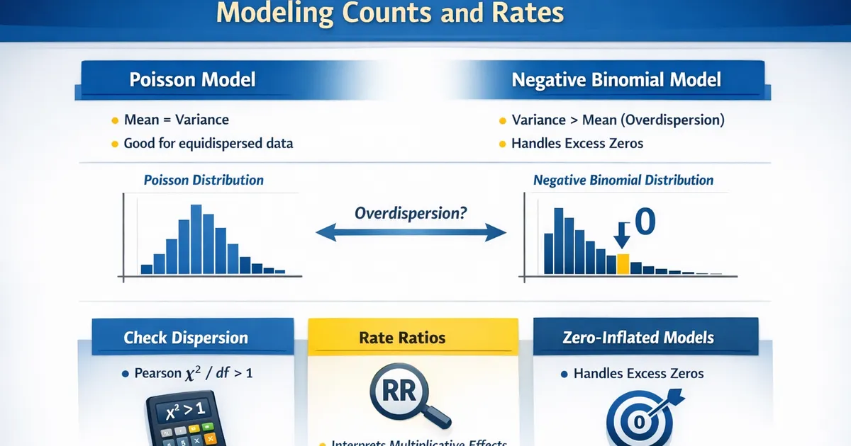
- •Poisson assumes mean equals variance - rarely true in real data
- •Negative binomial allows variance > mean (overdispersion)
- •Check dispersion: Pearson χ²/df >> 1 signals overdispersion
- •Rate ratios interpret as multiplicative changes in expected count
- •Zero-inflated models handle excess zeros from two processes
TL;DR
Count data (purchases, logins, support tickets) requires specialized regression methods. Poisson regression is the standard starting point, but it assumes variance equals the mean—rarely true in practice. When data shows overdispersion (variance > mean), negative binomial regression is preferred. Both produce rate ratios: multiplicative effects on expected counts. This guide shows how to choose between them, diagnose problems, and handle excess zeros.
When to Use Count Models
Use Poisson or negative binomial regression when your outcome is:
- A non-negative integer (0, 1, 2, 3, ...)
- A count of events (purchases, clicks, errors, messages)
- A rate when combined with an exposure/offset (events per time period)
Examples:
- Number of support tickets per user
- Number of purchases per month
- Number of app crashes per session
- Number of logins per week
Don't use when:
- Outcome is continuous → linear regression
- Outcome is binary → logistic regression
- Outcome is bounded (e.g., 0-5 rating) → ordinal regression
Poisson Regression
The Model
Or equivalently:
Key assumption: (variance equals mean)
Interpretation
= rate ratio (RR) for a one-unit increase in
Example: If , then
"For each additional unit of , the expected count is multiplied by 1.49 (a 49% increase)."
Adding an Offset (Exposure)
When observations have different exposure times:
Example: Users observed for different numbers of days
- User A: 10 purchases in 30 days
- User B: 5 purchases in 10 days
Without offset: User A looks more active With offset: User B has higher rate (0.5 vs 0.33 per day)
The Overdispersion Problem
What Is Overdispersion?
Overdispersion occurs when .
Common causes:
- Unobserved heterogeneity (hidden variation between individuals)
- Clustering (events cluster together)
- Correlation between events (one purchase leads to another)
Why It Matters
If you use Poisson with overdispersed data:
- Standard errors are too small
- P-values are too small
- Confidence intervals are too narrow
- You'll find too many "significant" effects
Detecting Overdispersion
Method 1: Dispersion statistic
- : Poisson is fine
-
1.5: Overdispersion likely
-
2: Definite overdispersion
Method 2: Compare mean and variance
For each level of predictors, is variance mean?
Method 3: Formal test
Cameron-Trivedi test for overdispersion:
- H₀: No overdispersion (Poisson is appropriate)
- Reject H₀ → use negative binomial
Negative Binomial Regression
The Model
Same mean structure as Poisson:
But with an extra dispersion parameter (or ):
When , this reduces to Poisson.
Interpretation
Coefficients interpret exactly like Poisson: is the rate ratio.
The difference is in the standard errors—negative binomial accounts for extra-Poisson variation.
When to Use
- Dispersion statistic > 1.5
- Variance clearly exceeds mean
- Likelihood ratio test rejects Poisson
- "To be safe" when you expect heterogeneity
Code: Poisson vs. Negative Binomial
Python
import numpy as np
import pandas as pd
import statsmodels.api as sm
import statsmodels.formula.api as smf
from scipy import stats


def compare_count_models(data, formula, exposure_col=None):
    """
    Fit Poisson and Negative Binomial, compare dispersion.

    Parameters:
    -----------
    data : pd.DataFrame
        Dataset
    formula : str
        Model formula (e.g., 'count ~ x1 + x2')
    exposure_col : str, optional
        Column name for exposure variable (for offset)

    Returns:
    --------
    dict with both models and comparison
    """
    results = {}

    # Fit Poisson
    if exposure_col:
        data['log_exposure'] = np.log(data[exposure_col])
        poisson_model = smf.poisson(
            formula,
            data=data,
            offset=data['log_exposure']
        ).fit(disp=0)
    else:
        poisson_model = smf.poisson(formula, data=data).fit(disp=0)

    results['poisson'] = poisson_model

    # Calculate dispersion statistic
    y_pred = poisson_model.predict()
    y_actual = poisson_model.model.endog
    pearson_resid = (y_actual - y_pred) / np.sqrt(y_pred)
    pearson_chi2 = np.sum(pearson_resid**2)
    df_resid = poisson_model.df_resid
    dispersion = pearson_chi2 / df_resid

    results['dispersion'] = {
        'pearson_chi2': pearson_chi2,
        'df_residual': df_resid,
        'dispersion_ratio': dispersion,
        'is_overdispersed': dispersion > 1.5
    }

    # Fit Negative Binomial
    if exposure_col:
        nb_model = smf.negativebinomial(
            formula,
            data=data,
            offset=data['log_exposure']
        ).fit(disp=0)
    else:
        nb_model = smf.negativebinomial(formula, data=data).fit(disp=0)

    results['negative_binomial'] = nb_model

    # Likelihood ratio test (Poisson vs NB)
    # Under H0: Poisson is adequate, the test statistic is chi-square with df=1
    lr_stat = 2 * (nb_model.llf - poisson_model.llf)
    lr_pvalue = stats.chi2.sf(lr_stat, 1)

    results['lr_test'] = {
        'statistic': lr_stat,
        'p_value': lr_pvalue,
        'prefer_nb': lr_pvalue < 0.05
    }

    # Model comparison
    results['comparison'] = pd.DataFrame({
        'Metric': ['Log-Likelihood', 'AIC', 'BIC'],
        'Poisson': [poisson_model.llf, poisson_model.aic, poisson_model.bic],
        'Neg. Binomial': [nb_model.llf, nb_model.aic, nb_model.bic]
    })

    return results


def get_rate_ratios(model, confidence=0.95):
    """Extract rate ratios with confidence intervals."""
    alpha = 1 - confidence
    z = stats.norm.ppf(1 - alpha/2)

    coef = model.params
    se = model.bse

    rate_ratios = pd.DataFrame({
        'Variable': coef.index,
        'Coefficient': coef.values,
        'Rate Ratio': np.exp(coef.values),
        'RR CI Lower': np.exp(coef.values - z * se.values),
        'RR CI Upper': np.exp(coef.values + z * se.values),
        'P-value': model.pvalues.values
    })

    return rate_ratios


def check_zero_inflation(data, outcome_col):
    """
    Check if data has excess zeros beyond Poisson expectation.
    """
    y = data[outcome_col]
    n = len(y)
    mean_y = y.mean()

    # Observed zero proportion
    obs_zeros = (y == 0).sum() / n

    # Expected zeros under Poisson
    exp_zeros = np.exp(-mean_y)

    return {
        'observed_zero_proportion': obs_zeros,
        'expected_zero_proportion_poisson': exp_zeros,
        'excess_zeros': obs_zeros > exp_zeros * 1.5,
        'ratio': obs_zeros / exp_zeros if exp_zeros > 0 else np.inf
    }


# Example usage
if __name__ == "__main__":
    np.random.seed(42)
    n = 500

    # Generate overdispersed count data
    # Using negative binomial to simulate
    from scipy.stats import nbinom

    data = pd.DataFrame({
        'segment': np.random.choice(['A', 'B', 'C'], n),
        'days_active': np.random.uniform(7, 90, n),
        'has_premium': np.random.binomial(1, 0.3, n)
    })

    # Generate counts with overdispersion
    mu = np.exp(0.5 + 0.3 * data['has_premium'] + 0.01 * data['days_active'])
    alpha = 0.5  # Overdispersion
    # Parameterize NB with mean mu and dispersion
    r = 1/alpha
    p = r / (r + mu)
    data['purchases'] = nbinom.rvs(r, p)

    # Compare models
    results = compare_count_models(data, 'purchases ~ has_premium + days_active')

    print("Count Model Comparison")
    print("=" * 60)
    print(f"\nDispersion ratio: {results['dispersion']['dispersion_ratio']:.2f}")
    print(f"Overdispersed: {results['dispersion']['is_overdispersed']}")
    print(f"\nLR test p-value: {results['lr_test']['p_value']:.4f}")
    print(f"Prefer NB: {results['lr_test']['prefer_nb']}")

    print("\n" + "=" * 60)
    print("Rate Ratios (Negative Binomial):")
    print(get_rate_ratios(results['negative_binomial']))

    # Check for zero inflation
    print("\n" + "=" * 60)
    zi = check_zero_inflation(data, 'purchases')
    print(f"Zero inflation check:")
    print(f"  Observed zeros: {zi['observed_zero_proportion']:.1%}")
    print(f"  Expected (Poisson): {zi['expected_zero_proportion_poisson']:.1%}")
    print(f"  Excess zeros: {zi['excess_zeros']}")
R
library(tidyverse)
library(MASS)  # For glm.nb
library(AER)   # For dispersiontest
library(pscl)  # For zero-inflated models


compare_count_models <- function(formula, data, exposure_col = NULL) {
    #' Compare Poisson and Negative Binomial models

    # Fit Poisson
    if (!is.null(exposure_col)) {
        data$log_exposure <- log(data[[exposure_col]])
        poisson_model <- glm(formula, data = data, family = poisson,
                            offset = log_exposure)
    } else {
        poisson_model <- glm(formula, data = data, family = poisson)
    }

    # Dispersion statistic
    pearson_chi2 <- sum(residuals(poisson_model, type = "pearson")^2)
    df_resid <- poisson_model$df.residual
    dispersion <- pearson_chi2 / df_resid

    # Formal dispersion test
    disp_test <- dispersiontest(poisson_model, trafo = 1)

    # Fit Negative Binomial
    if (!is.null(exposure_col)) {
        nb_model <- glm.nb(formula, data = data, offset = log_exposure)
    } else {
        nb_model <- glm.nb(formula, data = data)
    }

    # Likelihood ratio test
    lr_stat <- 2 * (logLik(nb_model) - logLik(poisson_model))
    lr_pvalue <- pchisq(as.numeric(lr_stat), 1, lower.tail = FALSE)

    list(
        poisson = poisson_model,
        negative_binomial = nb_model,
        dispersion = list(
            ratio = dispersion,
            test_p = disp_test$p.value,
            is_overdispersed = dispersion > 1.5 | disp_test$p.value < 0.05
        ),
        lr_test = list(
            statistic = as.numeric(lr_stat),
            p_value = lr_pvalue,
            prefer_nb = lr_pvalue < 0.05
        ),
        comparison = tibble(
            Model = c("Poisson", "Neg. Binomial"),
            LogLik = c(logLik(poisson_model), logLik(nb_model)),
            AIC = c(AIC(poisson_model), AIC(nb_model)),
            BIC = c(BIC(poisson_model), BIC(nb_model))
        )
    )
}


get_rate_ratios <- function(model) {
    #' Extract rate ratios with CIs

    coef_vals <- coef(model)
    se_vals <- summary(model)$coefficients[, "Std. Error"]
    ci <- confint(model)

    tibble(
        Variable = names(coef_vals),
        Coefficient = coef_vals,
        `Rate Ratio` = exp(coef_vals),
        `RR CI Lower` = exp(ci[, 1]),
        `RR CI Upper` = exp(ci[, 2]),
        `P-value` = summary(model)$coefficients[, "Pr(>|z|)"]
    )
}


# Example
set.seed(42)
n <- 500

data <- tibble(
    segment = sample(c("A", "B", "C"), n, replace = TRUE),
    days_active = runif(n, 7, 90),
    has_premium = rbinom(n, 1, 0.3)
) %>%
    mutate(
        mu = exp(0.5 + 0.3*has_premium + 0.01*days_active),
        purchases = rnbinom(n, size = 2, mu = mu)  # Overdispersed
    )

# Compare
results <- compare_count_models(purchases ~ has_premium + days_active, data)

cat("Count Model Comparison\n")
cat(strrep("=", 60), "\n")
cat(sprintf("Dispersion ratio: %.2f\n", results$dispersion$ratio))
cat(sprintf("Overdispersed: %s\n", results$dispersion$is_overdispersed))
cat(sprintf("\nLR test p-value: %.4f\n", results$lr_test$p_value))
cat(sprintf("Prefer NB: %s\n", results$lr_test$prefer_nb))

cat("\nRate Ratios (Negative Binomial):\n")
print(get_rate_ratios(results$negative_binomial))
Zero-Inflated Models
When Standard Models Fail
Sometimes you have more zeros than Poisson or negative binomial can explain:
Example: Number of purchases per user
- Many users never purchase (true zeros)
- Among purchasers, counts follow a distribution
- Two separate processes generate zeros
Zero-Inflated Poisson (ZIP)
Assumes two processes:
- With probability : always zero (structural zeros)
- With probability : Poisson-distributed counts (sampling zeros possible)
Zero-Inflated Negative Binomial (ZINB)
Same structure, but the count part follows negative binomial.
Code: Zero-Inflated Models
from statsmodels.discrete.count_model import ZeroInflatedPoisson, ZeroInflatedNegativeBinomialP

# Zero-inflated Poisson
zip_model = smf.poisson('count ~ x1 + x2', data=data)  # Standard first
# Note: statsmodels ZI models require different specification

# Using R is often easier for ZI models
library(pscl)

# Zero-inflated Poisson
zip_model <- zeroinfl(purchases ~ has_premium + days_active | 1,
                      data = data, dist = "poisson")

# Zero-inflated Negative Binomial
zinb_model <- zeroinfl(purchases ~ has_premium + days_active | 1,
                       data = data, dist = "negbin")

# Compare with Vuong test
vuong(zip_model, zinb_model)
When to Use Zero-Inflation
- Observed zeros >> expected zeros under Poisson/NB
- Theoretical reason for two zero-generating processes
- Vuong test suggests ZI model is better
Don't use if:
- Zeros are just low counts (no separate process)
- You don't have theoretical justification
Comparing Rates Across Groups
Rate Ratio Interpretation
If premium users have RR = 1.5:
- Premium users are expected to have 50% more events
- If baseline is 10 events, premium is 15 events
Comparing to a Reference
# In Python: first category is reference by default with C()
model = smf.negativebinomial('count ~ C(segment) + days', data=data).fit()

# Segment A is reference
# C(segment)[T.B] = rate ratio for B vs A
# C(segment)[T.C] = rate ratio for C vs A
Computing Incidence Rates
When you have exposure (time observed):
With an offset, coefficients give rate ratios directly.
Model Selection Decision Tree
START: Count outcome (0, 1, 2, ...)
       ↓
CHECK: Is there an exposure variable?
       ├── Yes → Include as offset
       └── No → Proceed
       ↓
FIT: Poisson model
       ↓
CHECK: Dispersion ratio
       ├── ≈ 1 → Poisson OK
       └── > 1.5 → Overdispersion
             ↓
       FIT: Negative Binomial
             ↓
CHECK: Excess zeros?
       ├── No → NB is final model
       └── Yes → Consider zero-inflated
             ↓
       FIT: ZIP or ZINB
       Compare with Vuong test
Summary Table
| Feature | Poisson | Negative Binomial | Zero-Inflated |
|---|---|---|---|
| Variance assumption | Two processes | ||
| Use when | Overdispersed | Excess zeros | |
| Standard errors | Can be too small | Appropriate | Appropriate |
| Interpretation | Rate ratios | Rate ratios | Two components |
| Complexity | Simple | Moderate | More complex |
Related Methods
- Regression for Analysts (Pillar) - Complete regression framework
- Comparing Rates - Rate comparisons without regression
- Dealing with Zeros - Zero-handling strategies
- Logistic Regression - Binary outcomes
Key Takeaway
For count data, start with Poisson but expect overdispersion. Check the dispersion ratio (Pearson χ²/df)—if it's above 1.5, switch to negative binomial. Both give rate ratios: multiplicative effects on expected counts. If you have more zeros than the model expects and there's a theoretical reason for two processes (never-purchasers vs. occasional-purchasers), consider zero-inflated models. Always interpret rate ratios correctly: RR = 1.5 means 50% more events, not "50% more likely."
References
- https://www.cambridge.org/core/books/regression-analysis-of-count-data/DC2FFD76B9AA7F3D7E62EA22DAC0AFB0
- https://bookdown.org/roback/bookdown-BeyondMLR/
- https://onlinelibrary.wiley.com/doi/10.1002/sim.3783
- Cameron, A. C., & Trivedi, P. K. (2013). Regression analysis of count data (2nd ed.). Cambridge University Press.
- Roback, P., & Legler, J. (2021). Beyond multiple linear regression: Applied generalized linear models and multilevel models in R. CRC Press.
- Hilbe, J. M. (2011). Negative binomial regression (2nd ed.). Cambridge University Press.
Frequently Asked Questions
When should I use Poisson vs. negative binomial?
What is overdispersion and why does it matter?
How do I interpret rate ratios?
Key Takeaway
Poisson regression is the starting point for count data, but overdispersion is common. Always check dispersion and use negative binomial when variance exceeds the mean. Both give rate ratios, which are multiplicative effects on expected counts.