Contents
Interaction Terms: When Treatment Effects Vary by Segment
A practical guide to interaction effects in regression. Learn when to include interactions, how to interpret them correctly, and common pitfalls when testing whether treatment effects differ across segments.
Quick Hits
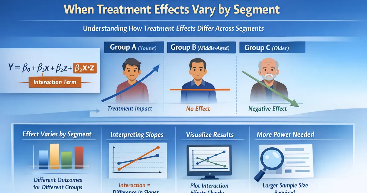
- •Interactions test whether one variable's effect depends on another variable's value
- •The interaction coefficient is the DIFFERENCE in slopes, not a separate effect
- •Main effects in interaction models mean something different than without interactions
- •Always visualize interactions - coefficients alone are hard to interpret
- •Testing for interaction requires more power than testing main effects
TL;DR
Interaction effects model whether one variable's effect depends on another variable. In A/B testing, this answers: "Does the treatment work differently for different segments?" The interaction coefficient represents the difference in treatment effects between groups, not a separate effect. Main effects with interactions have specific meanings (effect when moderator = 0), so center continuous moderators. Always visualize interactions—coefficient tables alone are hard to interpret.
What Interactions Model
Without Interaction
Meaning: X and Z have separate, additive effects on Y. The effect of X is regardless of Z's value.
With Interaction
Meaning: The effect of X depends on Z. Specifically:
- Effect of X when Z = 0:
- Effect of X when Z = 1:
- is the difference in effects
Coefficient Interpretation
Example: Treatment Premium User
Model:
| Coefficient | Interpretation |
|---|---|
| Mean revenue for Control, Non-Premium users | |
| Treatment effect for Non-Premium users | |
| Premium effect in Control group | |
| Additional treatment effect for Premium users |
Treatment effect for each group:
- Non-Premium:
- Premium:
Is the treatment effect different for Premium users? Test whether
Numerical Example
$\text{Revenue} = 50 + 10(\text{Treatment}) + 30(\text{Premium}) - 5(\text{Treatment} \times \text{Premium})$
| Group | Control | Treatment | Effect |
|---|---|---|---|
| Non-Premium | 50 | 60 | +10 |
| Premium | 80 | 85 | +5 |
The treatment lifts revenue by $10 for non-premium users, but only $5 for premium users. The interaction coefficient (-5) captures this difference.
The Main Effect Interpretation Problem
The Critical Point
In a model with interactions, main effects have conditional interpretations:
= effect of X when Z = 0
This is only meaningful if Z = 0 is a meaningful value!
Problem: Uncentered Continuous Moderator
Model: Conversion = Treatment + Age + Treatment × Age
- = treatment effect when Age = 0
- Age = 0 doesn't exist in your data → coefficient is meaningless
Solution: Center the Moderator
data['age_centered'] = data['age'] - data['age'].mean()
Now:
- = treatment effect at the average age
- This is interpretable and useful
Code: Interaction Models
Python
import numpy as np
import pandas as pd
import statsmodels.formula.api as smf
import matplotlib.pyplot as plt


def fit_interaction_model(data, outcome, treatment, moderator, is_categorical_moderator=False):
    """
    Fit a regression model with interaction and provide interpretable output.

    Parameters:
    -----------
    data : pd.DataFrame
        Dataset
    outcome : str
        Outcome variable name
    treatment : str
        Treatment variable name
    moderator : str
        Moderating variable name
    is_categorical_moderator : bool
        Whether moderator is categorical

    Returns:
    --------
    dict with model results and conditional effects
    """
    # Center continuous moderator if needed
    if not is_categorical_moderator:
        moderator_centered = f'{moderator}_centered'
        data[moderator_centered] = data[moderator] - data[moderator].mean()
        formula = f'{outcome} ~ {treatment} * {moderator_centered}'
    else:
        formula = f'{outcome} ~ {treatment} * C({moderator})'

    # Fit model
    model = smf.ols(formula, data=data).fit()

    results = {
        'model': model,
        'summary': model.summary(),
        'formula': formula
    }

    # Extract conditional effects
    if is_categorical_moderator:
        categories = data[moderator].unique()
        ref_category = sorted(categories)[0]  # First alphabetically is reference

        effects = {}
        treatment_coef = model.params[treatment]
        interaction_coefs = {k: v for k, v in model.params.items() if ':' in k}

        effects[ref_category] = {
            'effect': treatment_coef,
            'se': model.bse[treatment],
            'p_value': model.pvalues[treatment]
        }

        for cat in categories:
            if cat != ref_category:
                interaction_key = f'{treatment}:C({moderator})[T.{cat}]'
                if interaction_key in model.params:
                    effect = treatment_coef + model.params[interaction_key]
                    # Note: SE for sum requires covariance matrix
                    effects[cat] = {
                        'effect': effect,
                        'interaction_coef': model.params[interaction_key],
                        'interaction_p': model.pvalues[interaction_key]
                    }

        results['conditional_effects'] = effects
    else:
        # For continuous moderator: effect at mean, +/- 1 SD
        mean_mod = data[moderator].mean()
        sd_mod = data[moderator].std()

        treatment_at_mean = model.params[treatment]
        interaction_coef = model.params[f'{treatment}:{moderator_centered}']

        results['conditional_effects'] = {
            f'At mean {moderator}': treatment_at_mean,
            f'At mean - 1SD': treatment_at_mean - sd_mod * interaction_coef,
            f'At mean + 1SD': treatment_at_mean + sd_mod * interaction_coef
        }
        results['interaction_test'] = {
            'coefficient': interaction_coef,
            'p_value': model.pvalues[f'{treatment}:{moderator_centered}']
        }

    return results


def plot_interaction(data, outcome, treatment, moderator, model=None,
                    is_categorical=False, figsize=(10, 6)):
    """
    Visualize interaction effect.
    """
    fig, ax = plt.subplots(figsize=figsize)

    if is_categorical:
        # Bar plot for categorical moderator
        summary = data.groupby([moderator, treatment])[outcome].agg(['mean', 'sem']).reset_index()

        x = np.arange(len(data[moderator].unique()))
        width = 0.35

        control = summary[summary[treatment] == 0]
        treatment_df = summary[summary[treatment] == 1]

        ax.bar(x - width/2, control['mean'], width, yerr=control['sem']*1.96,
               label='Control', alpha=0.8, capsize=5)
        ax.bar(x + width/2, treatment_df['mean'], width, yerr=treatment_df['sem']*1.96,
               label='Treatment', alpha=0.8, capsize=5)

        ax.set_xticks(x)
        ax.set_xticklabels(control[moderator])
        ax.set_xlabel(moderator)
        ax.set_ylabel(outcome)
        ax.legend()

    else:
        # Scatter plot with regression lines for continuous moderator
        for treat_val, label, color in [(0, 'Control', 'blue'), (1, 'Treatment', 'orange')]:
            subset = data[data[treatment] == treat_val]
            ax.scatter(subset[moderator], subset[outcome], alpha=0.3, color=color, label=label)

            # Add regression line
            z = np.polyfit(subset[moderator], subset[outcome], 1)
            p = np.poly1d(z)
            x_line = np.linspace(subset[moderator].min(), subset[moderator].max(), 100)
            ax.plot(x_line, p(x_line), color=color, linewidth=2)

        ax.set_xlabel(moderator)
        ax.set_ylabel(outcome)
        ax.legend()

    ax.set_title(f'Interaction: {treatment} × {moderator}')
    plt.tight_layout()

    return fig


# Example usage
if __name__ == "__main__":
    np.random.seed(42)
    n = 500

    # Generate data with interaction
    data = pd.DataFrame({
        'treatment': np.random.binomial(1, 0.5, n),
        'segment': np.random.choice(['A', 'B', 'C'], n),
        'tenure_days': np.random.exponential(180, n)
    })

    # True model: treatment effect varies by segment
    base_effect = {'A': 10, 'B': 5, 'C': -2}
    data['revenue'] = (
        50 +
        data.apply(lambda r: base_effect[r['segment']] * r['treatment'], axis=1) +
        0.05 * data['tenure_days'] +
        np.random.normal(0, 15, n)
    )

    # Fit interaction model
    results = fit_interaction_model(
        data, 'revenue', 'treatment', 'segment',
        is_categorical_moderator=True
    )

    print("Interaction Model Results")
    print("=" * 60)
    print(results['summary'])
    print("\nConditional Effects:")
    for segment, effect in results['conditional_effects'].items():
        print(f"  {segment}: {effect}")

    # Visualize
    fig = plot_interaction(data, 'revenue', 'treatment', 'segment', is_categorical=True)
    plt.show()
R
library(tidyverse)
library(broom)
library(emmeans)  # For marginal means


fit_interaction_model <- function(data, formula, treatment, moderator) {
    #' Fit interaction model with interpretable output

    model <- lm(formula, data = data)

    # Get conditional effects using emmeans
    em <- emmeans(model, as.formula(paste("~", treatment, "|", moderator)))
    contrasts <- pairs(em)

    list(
        model = model,
        summary = summary(model),
        tidy = tidy(model, conf.int = TRUE),
        conditional_effects = contrasts,
        marginal_means = em
    )
}


plot_interaction <- function(data, outcome, treatment, moderator) {
    #' Visualize interaction

    summary_data <- data %>%
        group_by(across(all_of(c(treatment, moderator)))) %>%
        summarise(
            mean = mean(get(outcome)),
            se = sd(get(outcome)) / sqrt(n()),
            .groups = "drop"
        )

    ggplot(summary_data, aes_string(x = moderator, y = "mean",
                                     fill = paste0("factor(", treatment, ")"))) +
        geom_bar(stat = "identity", position = position_dodge(width = 0.8),
                 width = 0.7) +
        geom_errorbar(aes(ymin = mean - 1.96*se, ymax = mean + 1.96*se),
                      position = position_dodge(width = 0.8), width = 0.2) +
        labs(y = outcome, fill = treatment) +
        theme_minimal() +
        ggtitle(sprintf("Interaction: %s × %s", treatment, moderator))
}


# Example
set.seed(42)
n <- 500

data <- tibble(
    treatment = rbinom(n, 1, 0.5),
    segment = sample(c("A", "B", "C"), n, replace = TRUE),
    tenure_days = rexp(n, 1/180)
) %>%
    mutate(
        effect = case_when(
            segment == "A" ~ 10,
            segment == "B" ~ 5,
            segment == "C" ~ -2
        ),
        revenue = 50 + effect * treatment + 0.05 * tenure_days + rnorm(n, 0, 15)
    )

# Fit model
results <- fit_interaction_model(
    data,
    revenue ~ treatment * segment,
    "treatment",
    "segment"
)

cat("Model Summary:\n")
print(results$tidy)

cat("\nConditional Effects:\n")
print(results$conditional_effects)

# Plot
plot_interaction(data, "revenue", "treatment", "segment")
Power for Interaction Tests
The Uncomfortable Truth
Detecting interactions requires substantially more power than detecting main effects.
Rule of thumb: To detect an interaction with the same power as a main effect, you need 4× the sample size.
Why?
The interaction tests whether the difference in effects is significant. You're essentially estimating and comparing two effects, which compounds the uncertainty.
Implications
- Many "no interaction" findings are underpowered: Absence of significant interaction effects are equal
- Plan studies specifically for interaction detection: If you want to test heterogeneity, power for it explicitly
- Consider Bayesian approaches: To distinguish "no difference" from "insufficient evidence"
Common Mistakes
Mistake 1: Interpreting Main Effects Without Context
Wrong: "Treatment has a significant main effect of +5"
When there's an interaction: The main effect of +5 is only the treatment effect when the moderator = 0 (or reference category).
Right: "Treatment effect is +5 in the reference group (Segment A), and varies by segment"
Mistake 2: Running Separate Regressions Instead of Interaction
What analysts do: Run regression separately for each segment, compare coefficients
Problems:
- No formal test of whether coefficients differ
- Less statistical power
- Doesn't account for shared parameters
Better: Use interaction model, test interaction coefficient
Mistake 3: Including Too Many Interactions
Temptation: Test treatment everything
Problem: Multiple comparisons inflate false positive rate
Better:
- Pre-specify which interactions to test
- Apply multiple comparison corrections
- Focus on theoretically motivated interactions
Mistake 4: Confusing Interaction with Non-Linear Main Effect
Sometimes what looks like an interaction is really a non-linear effect of one variable.
Check: Does including X² reduce/eliminate the "interaction"?
Types of Interactions
Ordinal vs. Disordinal
Ordinal (same direction, different magnitude):
- Treatment helps both groups, but helps one more
- Lines don't cross
Disordinal (different directions):
- Treatment helps one group, hurts another
- Lines cross
Quantitative vs. Qualitative
Quantitative: Treatment effect exists in both groups, but varies in size
Qualitative: Treatment effect reverses direction between groups (e.g., +10 in one, -5 in another)
Qualitative interactions are rarer but more important—they suggest treatment should be targeted.
Testing for Interaction: Decision Guide
When to Include Interaction Terms
- Theoretical reason: You expect effects to vary
- Prior evidence: Literature suggests heterogeneity
- Pre-registered: You planned to test it
- Sufficient power: You have sample size for interaction detection
When NOT to Include
- Fishing expedition: Testing every possible interaction
- Underpowered: Can't detect reasonable interaction sizes
- Post-hoc: Adding after seeing surprising subgroup differences
- No interpretation: No theory for why effects would vary
Reporting Guidelines
- Report main effects model first
- Add interaction and test formally
- Show conditional effects for each level
- Visualize the interaction
- Acknowledge power limitations
Interactions in Logistic Regression
Interactions in logistic regression are on the log-odds scale:
Interpretation: is the ratio of odds ratios
Example: OR for treatment in non-premium = 1.5, OR in premium = 2.25
- Interaction OR = 2.25/1.5 = 1.5
- "The treatment odds ratio is 50% higher for premium users"
Note: Interaction on odds scale interaction on probability scale
Related Methods
- Regression for Analysts (Pillar) - Complete regression framework
- Two-Way ANOVA vs. Regression - ANOVA interaction perspective
- Multiple Comparisons - Correcting for multiple interactions
- Subgroup Analysis Pitfalls - Post-hoc interaction dangers
Key Takeaway
Interactions model whether one variable's effect depends on another. The interaction coefficient is the difference in effects between groups, not a standalone effect. Main effects in interaction models have conditional interpretations (effect when moderator = 0), so center continuous moderators. Always visualize—coefficient tables hide the pattern. And remember: detecting interactions requires 4× the sample size of main effects, so many "null" interaction tests are simply underpowered.
References
- https://journals.sagepub.com/doi/10.1177/1094428114568020
- https://www.ncbi.nlm.nih.gov/pmc/articles/PMC4372376/
- https://doi.org/10.1037/met0000227
- McClelland, G. H., & Judd, C. M. (1993). Statistical difficulties of detecting interactions and moderator effects. *Psychological Bulletin*, 114(2), 376-390.
- Rohrer, J. M., & Arslan, R. C. (2021). Precise answers to vague questions: Issues with interactions. *Advances in Methods and Practices in Psychological Science*, 4(2).
- Gelman, A. (2018). You need 16 times the sample size to estimate an interaction than to estimate a main effect. *Statistical Modeling, Causal Inference, and Social Science* (blog).
Frequently Asked Questions
What's the difference between interaction and confounding?
How do I interpret main effects when there's an interaction?
Why can't I just run separate regressions for each segment?
Key Takeaway
Interaction terms answer: 'Does the effect of X on Y depend on the value of Z?' The interaction coefficient is the difference in slopes between groups, not a separate effect. Always center continuous moderators, always visualize, and remember that detecting interactions requires substantially more statistical power than detecting main effects.