Contents
Independence: The Silent Killer of Statistical Validity
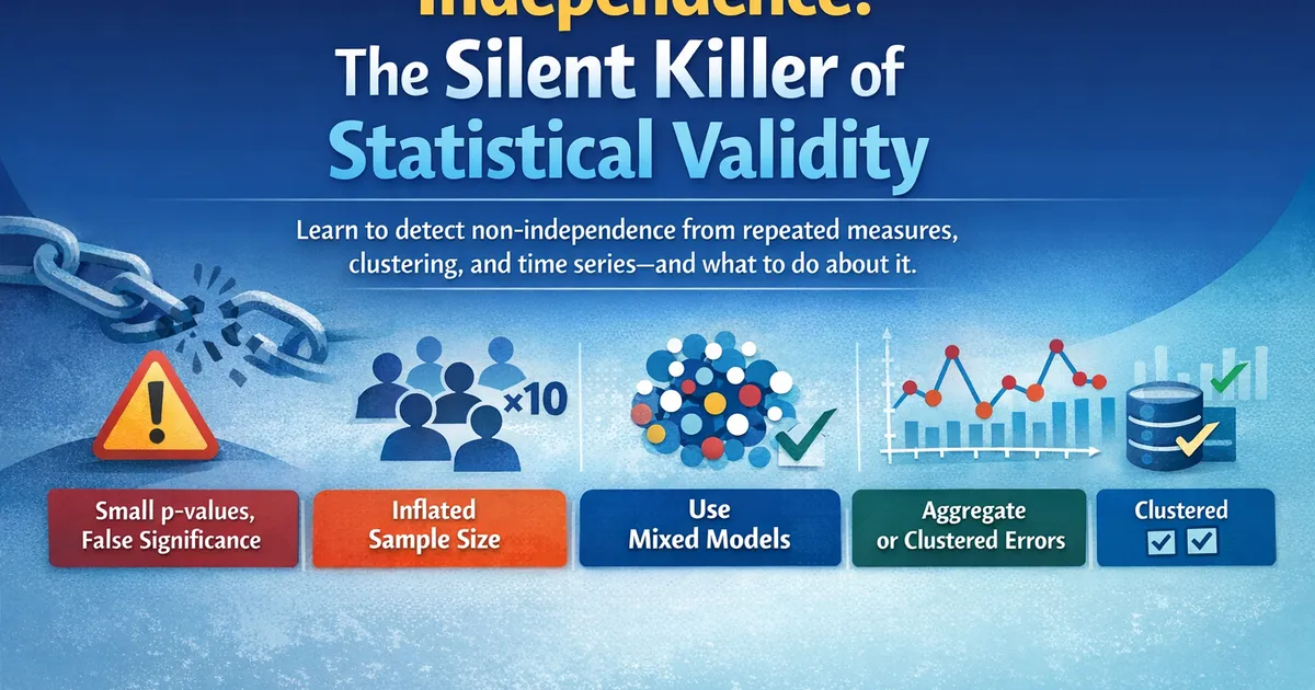
The independence assumption is the most critical and most commonly violated. Learn to detect non-independence from repeated measures, clustering, and time series—and what to do about it.
Quick Hits
- •Independence violations can't be fixed with robust methods—they require structural solutions
- •Multiple observations per user is the most common violation in product analytics
- •Ignoring clustering can inflate effective sample size by 10x or more
- •Solutions include mixed models, clustered standard errors, or aggregation
TL;DR
Independence violations are the most dangerous assumption problems because they can't be fixed with robust methods. When observations are correlated (repeated measures, clustering, time series), standard errors shrink artificially, making everything look more significant than it is. The solutions require restructuring your analysis: aggregate to independent units, use clustered standard errors, or fit models that account for the correlation structure.
What Independence Means
The Formal Definition
Observations are independent if knowing the value of one tells you nothing about another:
Practical Translation
Ask yourself: "If I know user A's value, does that help me predict user B's value?"
- Independent: Different users randomly sampled from different sources
- Not independent: Multiple purchases from the same user, students in the same classroom, time-series data
| Violation | Example | Why problematic | Effective n |
|---|---|---|---|
| Repeated measures | Multiple sessions/purchases per user | Users are consistent with themselves | Much smaller than observation count |
| Clustering | Users in same company, classroom, region | Within-cluster similarity | Closer to number of clusters than observations |
| Time series | Daily/weekly metrics | Autocorrelation — today predicts tomorrow | Depends on correlation structure |
| Network effects | Users who interact with each other | Treatment spreads through network | May need network randomization |
| Spatial correlation | Users in nearby locations | Geographic similarity | Depends on spatial structure |
The Damage: Inflated Type I Error
Simulation: How Bad Can It Get?
import numpy as np
from scipy import stats
import pandas as pd

def simulate_clustering_damage(n_sims=5000):
    """
    Show how clustering inflates Type I error.
    """
    np.random.seed(42)

    # Scenario: 20 clusters of 10 observations each = 200 total
    n_clusters = 20
    cluster_size = 10
    n_total = n_clusters * cluster_size

    # Vary intraclass correlation (ICC)
    iccs = [0, 0.1, 0.3, 0.5, 0.7]

    results = {}
    for icc in iccs:
        # ICC determines how much variance is between vs within clusters
        between_var = icc
        within_var = 1 - icc

        rejections_naive = 0
        rejections_clustered = 0

        for _ in range(n_sims):
            # Generate null data (no treatment effect)
            data = []
            for cluster in range(n_clusters):
                # Half clusters are "treatment", half are "control"
                treatment = cluster >= n_clusters // 2
                cluster_effect = np.random.normal(0, np.sqrt(between_var))

                for _ in range(cluster_size):
                    obs = cluster_effect + np.random.normal(0, np.sqrt(within_var))
                    data.append({
                        'cluster': cluster,
                        'treatment': treatment,
                        'value': obs
                    })

            df = pd.DataFrame(data)

            # Naive analysis (ignores clustering)
            control = df[~df['treatment']]['value']
            treat = df[df['treatment']]['value']
            _, p_naive = stats.ttest_ind(control, treat)
            if p_naive < 0.05:
                rejections_naive += 1

            # Correct analysis (cluster means)
            cluster_means = df.groupby(['treatment', 'cluster'])['value'].mean()
            control_means = cluster_means[False].values
            treat_means = cluster_means[True].values
            _, p_correct = stats.ttest_ind(control_means, treat_means)
            if p_correct < 0.05:
                rejections_clustered += 1

        results[icc] = {
            'naive': rejections_naive / n_sims,
            'correct': rejections_clustered / n_sims
        }

    print("Type I Error with Clustered Data (α = 0.05)")
    print("=" * 50)
    print(f"{'ICC':>6} {'Naive':>12} {'Clustered':>12} {'Inflation':>12}")
    print("-" * 50)
    for icc, res in results.items():
        inflation = res['naive'] / 0.05
        print(f"{icc:>6.1f} {res['naive']:>12.3f} {res['correct']:>12.3f} {inflation:>11.1f}x")

    return results


simulate_clustering_damage()
What's Actually Happening
With clustering, your effective sample size is:
Where = total observations, = average cluster size, and = intraclass correlation.
For example, with 1,000 purchases from 100 users (m = 10 each):
| ICC | Effective n |
|---|---|
| 0.1 | 526 |
| 0.3 | 270 |
| 0.5 | 182 |
| 0.7 | 137 |
Even moderate ICC dramatically reduces the effective sample size compared to the raw 1,000 observations.
Detecting Non-Independence
Check 1: Data Structure
def check_data_structure(df, unit_col, observation_col=None):
    """
    Identify potential independence violations from data structure.
    """
    # Count observations per unit
    obs_per_unit = df.groupby(unit_col).size()

    results = {
        'total_observations': len(df),
        'unique_units': df[unit_col].nunique(),
        'obs_per_unit': {
            'mean': obs_per_unit.mean(),
            'median': obs_per_unit.median(),
            'max': obs_per_unit.max(),
            'min': obs_per_unit.min()
        },
        'units_with_multiple': (obs_per_unit > 1).sum(),
        'pct_from_repeat_units': (obs_per_unit[obs_per_unit > 1].sum() /
                                   len(df) * 100 if (obs_per_unit > 1).any() else 0)
    }

    # Diagnosis
    if results['obs_per_unit']['mean'] > 1.5:
        results['warning'] = (
            f"⚠️  Average of {results['obs_per_unit']['mean']:.1f} observations per unit. "
            f"Independence is likely violated."
        )

    return results


# Example
np.random.seed(42)
n_users = 50
data = []
for user in range(n_users):
    n_sessions = np.random.poisson(5) + 1
    for session in range(n_sessions):
        data.append({
            'user_id': user,
            'session_value': np.random.normal(100, 20)
        })

df = pd.DataFrame(data)
structure = check_data_structure(df, 'user_id')

print("Data Structure Analysis:")
print("-" * 40)
print(f"Total observations: {structure['total_observations']}")
print(f"Unique users: {structure['unique_units']}")
print(f"Mean obs per user: {structure['obs_per_unit']['mean']:.1f}")
print(f"Max obs per user: {structure['obs_per_unit']['max']}")
if 'warning' in structure:
    print(f"\n{structure['warning']}")
Check 2: Intraclass Correlation (ICC)
def calculate_icc(df, group_col, value_col):
    """
    Calculate intraclass correlation coefficient.
    """
    # Get group means and sizes
    groups = df.groupby(group_col)[value_col]
    group_means = groups.mean()
    group_sizes = groups.size()
    grand_mean = df[value_col].mean()

    n_groups = len(group_means)
    n_total = len(df)
    avg_size = n_total / n_groups

    # Between-group variance
    ss_between = sum(group_sizes * (group_means - grand_mean)**2)
    ms_between = ss_between / (n_groups - 1)

    # Within-group variance
    ss_within = sum(groups.apply(lambda x: sum((x - x.mean())**2)))
    ms_within = ss_within / (n_total - n_groups)

    # ICC (one-way random effects)
    icc = (ms_between - ms_within) / (ms_between + (avg_size - 1) * ms_within)
    icc = max(0, icc)  # Can't be negative

    # Effective sample size
    n_eff = n_total / (1 + (avg_size - 1) * icc)

    return {
        'icc': icc,
        'n_total': n_total,
        'n_groups': n_groups,
        'avg_group_size': avg_size,
        'effective_n': n_eff,
        'design_effect': 1 + (avg_size - 1) * icc
    }


# Calculate ICC for our example
icc_result = calculate_icc(df, 'user_id', 'session_value')

print("Intraclass Correlation Analysis:")
print("-" * 40)
print(f"ICC: {icc_result['icc']:.3f}")
print(f"Total observations: {icc_result['n_total']}")
print(f"Effective sample size: {icc_result['effective_n']:.0f}")
print(f"Design effect: {icc_result['design_effect']:.1f}")
Check 3: Autocorrelation (Time Series)
from scipy.stats import pearsonr

def check_autocorrelation(series, max_lag=5):
    """
    Check for autocorrelation in time series data.
    """
    series = np.array(series)
    n = len(series)

    results = {'lags': []}
    for lag in range(1, min(max_lag + 1, n // 4)):
        corr, p = pearsonr(series[:-lag], series[lag:])
        results['lags'].append({
            'lag': lag,
            'correlation': corr,
            'p_value': p
        })

    # Durbin-Watson statistic
    residuals = series - np.mean(series)
    dw = np.sum(np.diff(residuals)**2) / np.sum(residuals**2)
    results['durbin_watson'] = dw
    # DW ≈ 2 means no autocorrelation
    # DW < 2 means positive autocorrelation
    # DW > 2 means negative autocorrelation

    return results


# Example: Daily metrics
np.random.seed(42)
daily_metric = np.cumsum(np.random.normal(0.1, 1, 100)) + 100  # Random walk

auto_result = check_autocorrelation(daily_metric)
print("Autocorrelation Check:")
print("-" * 40)
print(f"Durbin-Watson: {auto_result['durbin_watson']:.2f} (2 = no autocorrelation)")
print("\nLag correlations:")
for lag_info in auto_result['lags'][:3]:
    print(f"  Lag {lag_info['lag']}: r = {lag_info['correlation']:.3f}, "
          f"p = {lag_info['p_value']:.4f}")
Solutions
Solution 1: Aggregate to Independent Units
The simplest solution: collapse data to one observation per independent unit.
def aggregate_solution(df, unit_col, value_col, group_col=None):
    """
    Aggregate to unit level to restore independence.
    """
    if group_col:
        # Aggregate within groups
        aggregated = df.groupby([group_col, unit_col]).agg({
            value_col: ['mean', 'std', 'count']
        }).reset_index()
        aggregated.columns = [group_col, unit_col, 'mean', 'std', 'n_obs']
    else:
        aggregated = df.groupby(unit_col).agg({
            value_col: ['mean', 'std', 'count']
        }).reset_index()
        aggregated.columns = [unit_col, 'mean', 'std', 'n_obs']

    return aggregated


# Example: Compare treatment vs control
np.random.seed(42)
data = []
for user in range(100):
    treatment = user >= 50
    user_effect = np.random.normal(0, 5)
    treatment_effect = 3 if treatment else 0

    for session in range(np.random.poisson(5) + 1):
        data.append({
            'user_id': user,
            'treatment': treatment,
            'value': 50 + user_effect + treatment_effect + np.random.normal(0, 10)
        })

df = pd.DataFrame(data)

# Wrong: observation-level analysis
control_obs = df[~df['treatment']]['value']
treat_obs = df[df['treatment']]['value']
_, p_wrong = stats.ttest_ind(control_obs, treat_obs)

# Right: user-level analysis
user_means = df.groupby(['treatment', 'user_id'])['value'].mean().reset_index()
control_users = user_means[~user_means['treatment']]['value']
treat_users = user_means[user_means['treatment']]['value']
_, p_right = stats.ttest_ind(control_users, treat_users)

print("Impact of Aggregation:")
print("-" * 40)
print(f"Observation-level (WRONG): n = {len(df)}, p = {p_wrong:.4f}")
print(f"User-level (RIGHT): n = {len(user_means)}, p = {p_right:.4f}")
Solution 2: Clustered Standard Errors
For regression, adjust standard errors to account for clustering.
import statsmodels.api as sm

def clustered_regression(df, outcome_col, predictor_cols, cluster_col):
    """
    Regression with clustered standard errors.
    """
    y = df[outcome_col]
    X = sm.add_constant(df[predictor_cols])

    # Standard OLS
    model_standard = sm.OLS(y, X).fit()

    # With clustered standard errors
    model_clustered = sm.OLS(y, X).fit(cov_type='cluster',
                                        cov_kwds={'groups': df[cluster_col]})

    return model_standard, model_clustered


# Example
np.random.seed(42)

# Create clustered data with treatment effect
data = []
for cluster in range(50):
    treatment = cluster >= 25
    cluster_effect = np.random.normal(0, 10)

    for _ in range(np.random.poisson(10) + 1):
        value = 50 + cluster_effect + (5 if treatment else 0) + np.random.normal(0, 5)
        data.append({
            'cluster': cluster,
            'treatment': int(treatment),
            'value': value
        })

df = pd.DataFrame(data)

model_std, model_clust = clustered_regression(df, 'value', ['treatment'], 'cluster')

print("Regression Results Comparison:")
print("-" * 50)
print(f"{'':20} {'Standard SE':>15} {'Clustered SE':>15}")
print("-" * 50)

for var in ['const', 'treatment']:
    se_std = model_std.bse[var]
    se_clust = model_clust.bse[var]
    ratio = se_clust / se_std
    print(f"{var:20} {se_std:>15.3f} {se_clust:>15.3f} ({ratio:.1f}x)")

print("\nP-values for treatment:")
print(f"  Standard: {model_std.pvalues['treatment']:.4f}")
print(f"  Clustered: {model_clust.pvalues['treatment']:.4f}")
Solution 3: Mixed Effects Models
For complex structures, use multilevel/mixed models.
import statsmodels.formula.api as smf

def mixed_model_analysis(df, outcome, fixed_effects, random_effects):
    """
    Fit mixed effects model.
    """
    formula = f"{outcome} ~ {fixed_effects}"
    model = smf.mixedlm(formula, df, groups=random_effects).fit()
    return model


# Example: Users nested in companies
np.random.seed(42)
data = []
for company in range(20):
    company_effect = np.random.normal(0, 10)
    treatment = company >= 10

    for user in range(np.random.randint(5, 15)):
        user_effect = np.random.normal(0, 5)

        for session in range(np.random.poisson(3) + 1):
            value = (50 + company_effect + user_effect +
                    (5 if treatment else 0) + np.random.normal(0, 3))
            data.append({
                'company': company,
                'user': f"{company}_{user}",
                'treatment': int(treatment),
                'value': value
            })

df = pd.DataFrame(data)

# Fit mixed model (random intercept for company)
model = smf.mixedlm("value ~ treatment", df, groups="company").fit()

print("Mixed Model Results:")
print("-" * 50)
print(model.summary().tables[1])
Decision Framework
Do observations repeat within units (users, clusters, time)?
│
├── NO → Standard methods OK
│
└── YES → How to handle?
          │
          ├── Simple structure (one observation per unit possible)?
          │   └── Aggregate to unit means
          │
          ├── Need observation-level analysis?
          │   ├── Regression → Clustered standard errors
          │   └── Complex nesting → Mixed effects models
          │
          └── Time series?
              └── Time series methods (ARIMA, etc.)
R Implementation
# Check for clustering
check_clustering <- function(df, unit_col, value_col) {
  library(ICC)

  # ICC calculation
  icc_result <- ICCbare(unit_col, value_col, data = df)

  # Effective sample size
  n_total <- nrow(df)
  n_units <- length(unique(df[[unit_col]]))
  avg_size <- n_total / n_units
  n_eff <- n_total / (1 + (avg_size - 1) * icc_result)

  cat("Independence Check\n")
  cat(rep("=", 40), "\n")
  cat(sprintf("Total observations: %d\n", n_total))
  cat(sprintf("Unique units: %d\n", n_units))
  cat(sprintf("ICC: %.3f\n", icc_result))
  cat(sprintf("Effective n: %.0f\n", n_eff))
}

# Clustered standard errors
library(sandwich)
library(lmtest)

model <- lm(value ~ treatment, data = df)
coeftest(model, vcov = vcovCL(model, cluster = df$cluster))

# Mixed effects model
library(lme4)
model <- lmer(value ~ treatment + (1|cluster), data = df)
summary(model)
Related Methods
- Assumption Checks Master Guide — The pillar article
- Clustered Experiments — A/B tests with clustering
- Paired vs. Independent Data — When data is paired
Key Takeaway
Independence is the most critical assumption because violations cannot be fixed with robust methods. When observations are clustered (repeated measures, grouped data, time series), your effective sample size is smaller than your observation count—sometimes dramatically so. The solutions require structural changes: aggregate to independent units, use clustered standard errors, or fit mixed models. Always ask: "Are my observations truly independent?"
References
- https://www.jstor.org/stable/2531734
- https://doi.org/10.1037/a0014694
- Aarts, E., Verhage, M., Veenvliet, J. V., Dolan, C. V., & Van Der Sluis, S. (2014). A solution to dependency: using multilevel analysis to accommodate nested data. *Nature Neuroscience*, 17(4), 491-496.
- Moulton, B. R. (1986). Random group effects and the precision of regression estimates. *Journal of Econometrics*, 32(3), 385-397.
- Snijders, T. A., & Bosker, R. J. (2011). *Multilevel Analysis: An Introduction to Basic and Advanced Multilevel Modeling* (2nd ed.). Sage.
Frequently Asked Questions
What happens if I ignore non-independence?
Can I just use a robust test to fix this?
How do I know if my data is independent?
Key Takeaway
Independence is the most important and most commonly violated assumption. Unlike normality or equal variance, violations cannot be fixed by using robust methods—they require fundamentally different approaches: aggregating to independent units, using clustered standard errors, or fitting mixed/multilevel models.