Contents
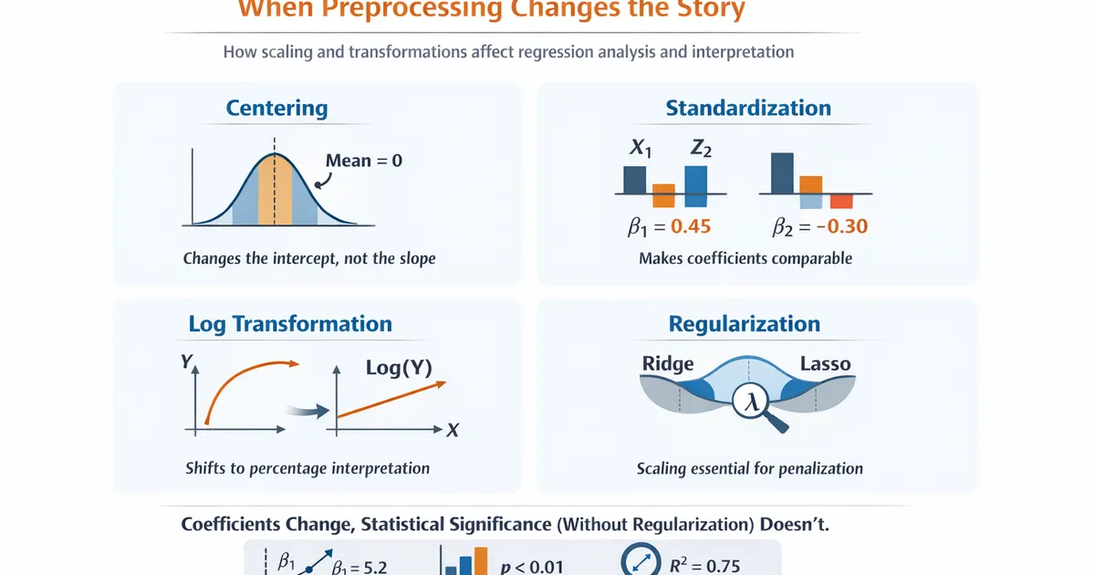
Feature Scaling and Transforms: When Preprocessing Changes the Story
A practical guide to standardization, centering, and transformations in regression. Learn when scaling affects interpretation, when it's required, and how to interpret coefficients on transformed variables.
Quick Hits
- •Centering changes intercept interpretation but not slopes
- •Standardizing makes coefficients comparable across variables
- •Log transforms change interpretation to percentage/elasticity terms
- •For linear regression without regularization, scaling doesn't affect significance
- •For ridge/lasso, scaling is essential - it affects which variables get penalized
TL;DR
How you scale and transform variables affects how you interpret regression coefficients, but for standard OLS, it doesn't change p-values or overall model fit. Centering makes the intercept meaningful, standardizing enables comparing coefficient magnitudes, and log transforms shift interpretation to percentage terms. For regularized regression (ridge, lasso), scaling is essential—it determines which variables get penalized more.
The Key Distinction
What scaling changes:
- Coefficient values
- Intercept value
- Interpretation of coefficients
What scaling doesn't change (in OLS without regularization):
- t-statistics
- p-values
- R² and adjusted R²
- Predictions
- Overall model fit
Centering: Moving the Origin
What Centering Does
Centering subtracts the mean from each variable:
Effect on Coefficients
| Term | Before Centering | After Centering |
|---|---|---|
| Intercept | Value of Y when X = 0 | Value of Y when X = mean(X) |
| Slope | Unchanged | Unchanged |
When to Center
-
Making the intercept interpretable: If X = 0 is impossible (e.g., age), centering makes the intercept meaningful
-
Reducing collinearity with interactions: Centering X before creating reduces correlation between main effects and interactions
-
Numerical stability: For very large values, centering can improve computation
Code: Centering
import pandas as pd
import numpy as np

# Center a variable
data['age_centered'] = data['age'] - data['age'].mean()

# Center multiple variables
for col in ['age', 'income', 'tenure']:
    data[f'{col}_centered'] = data[col] - data[col].mean()
# Center a variable
data$age_centered <- data$age - mean(data$age)

# Or using scale
data$age_centered <- scale(data$age, center = TRUE, scale = FALSE)
Standardization: Making Variables Comparable
What Standardization Does
Standardization creates z-scores (mean = 0, SD = 1):
Effect on Coefficients
Before: β = change in Y for a one-unit change in X
After: β = change in Y for a one-SD change in X
This makes coefficients comparable across variables with different scales.
Example
| Variable | Unstandardized β | SD | Standardized β |
|---|---|---|---|
| Age (years) | 500 | 10 | 5,000 |
| Income ($) | 0.01 | 50,000 | 500 |
Without standardization, income's coefficient looks small (0.01). With standardization, we see age has 10× the effect per SD.
When to Standardize
-
Comparing coefficient magnitudes: "Which variable has the bigger effect?"
-
Regularized regression: Ridge/lasso penalize coefficients—without standardization, variables with large scales are unfairly penalized
-
When units are arbitrary: Survey items (1-5 vs 1-100 scales) have arbitrary units
When NOT to Standardize
-
When natural units are meaningful: "Each additional year of education increases salary by $5,000" is clearer than "Each SD of education..."
-
When comparing across studies: Standardized coefficients depend on your sample's variance
Code: Standardization
import numpy as np
from sklearn.preprocessing import StandardScaler

# Manual
data['age_std'] = (data['age'] - data['age'].mean()) / data['age'].std()

# Using sklearn (for ML pipelines)
scaler = StandardScaler()
data[['age_std', 'income_std']] = scaler.fit_transform(data[['age', 'income']])
# Using scale()
data$age_std <- scale(data$age)  # Centers and scales by default

# Manual
data$age_std <- (data$age - mean(data$age)) / sd(data$age)
Log Transformations: Multiplicative Effects
When to Log-Transform
Log-transform the outcome when:
- Outcome is strictly positive
- Outcome is right-skewed (revenue, income, time)
- You want to model multiplicative/percentage effects
- Residuals from linear model are heteroscedastic
Log-transform predictors when:
- Predictor is strictly positive and right-skewed
- You expect diminishing marginal effects (doubling X doesn't double effect)
- The relationship is multiplicative
Interpretation Guide
| Model | Coefficient Interpretation |
|---|---|
| = change in for 1-unit change in | |
| change in for 1-unit change in (approx.) | |
| = change in for 1% change in | |
| = elasticity (% change in for 1% change in ) |
Example: Log-Linear Model
Model:
Interpretation: Each additional email is associated with approximately 3% higher revenue.
More precise: The multiplier is , so exactly 3.05% higher.
Example: Log-Log Model (Elasticity)
Model:
Interpretation: A 1% increase in advertising is associated with a 0.8% increase in sales. (Elasticity = 0.8)
Code: Log Transformations
import numpy as np

# Log transform (handling zeros)
data['log_revenue'] = np.log(data['revenue'] + 1)  # Add 1 if zeros present
data['log_revenue'] = np.log(data['revenue'])      # If no zeros

# Log-linear model
import statsmodels.formula.api as smf
model = smf.ols('np.log(revenue) ~ emails + premium', data=data).fit()

# Interpret coefficient
coef = model.params['emails']
pct_change = (np.exp(coef) - 1) * 100
print(f"Each email associated with {pct_change:.1f}% change in revenue")
# Log transform
data$log_revenue <- log(data$revenue)
data$log_revenue <- log(data$revenue + 1)  # If zeros present

# Log-linear model
model <- lm(log(revenue) ~ emails + premium, data = data)

# Interpret
coef <- coef(model)["emails"]
pct_change <- (exp(coef) - 1) * 100
cat(sprintf("Each email associated with %.1f%% change in revenue\n", pct_change))
Other Common Transformations
Square Root
Use when: Count data with many small values, moderate right skew.
Interpretation: Harder than log—1-unit change in corresponds to different X changes at different levels.
Box-Cox
Finds the optimal power transformation:
Use when: You want to normalize residuals/improve linearity and don't care about interpretation.
from scipy import stats

# Find optimal lambda
transformed_y, lambda_opt = stats.boxcox(data['y'])
print(f"Optimal lambda: {lambda_opt}")
Inverse
Use when: Relationship is hyperbolic (e.g., speed vs. time, rate × time = distance).
Scaling and Regularization
Why Scaling Matters for Ridge/Lasso
Regularization adds a penalty on coefficient size:
- Ridge:
- Lasso:
Problem: Without scaling, variables with larger values have smaller coefficients (in original units), so they're penalized less.
Example:
- Age coefficient: 500 (age in years, range 20-70)
- Income coefficient: 0.001 (income in dollars, range 20,000-200,000)
Ridge penalty of 500² >> 0.001², so age gets penalized much more—but that's just a unit artifact.
Always Standardize for Regularized Regression
from sklearn.preprocessing import StandardScaler
from sklearn.linear_model import Ridge

# Scale first
scaler = StandardScaler()
X_scaled = scaler.fit_transform(X)

# Then fit
ridge = Ridge(alpha=1.0)
ridge.fit(X_scaled, y)
Code: Complete Preprocessing Workflow
Python
import numpy as np
import pandas as pd
import statsmodels.formula.api as smf
from sklearn.preprocessing import StandardScaler


def preprocess_for_regression(data, outcome, predictors,
                              center=None, standardize=None,
                              log_transform=None):
    """
    Preprocess variables for regression with clear interpretation.

    Parameters:
    -----------
    data : pd.DataFrame
        Dataset
    outcome : str
        Outcome variable name
    predictors : list
        Predictor variable names
    center : list, optional
        Variables to center
    standardize : list, optional
        Variables to standardize
    log_transform : list, optional
        Variables to log-transform

    Returns:
    --------
    Preprocessed DataFrame and interpretation guide
    """
    df = data.copy()
    interpretations = {}

    # Centering
    if center:
        for var in center:
            mean_val = df[var].mean()
            df[f'{var}_c'] = df[var] - mean_val
            interpretations[f'{var}_c'] = (
                f"Centered at mean={mean_val:.2f}. "
                f"Coefficient = effect of 1-unit change in {var}"
            )

    # Standardization
    if standardize:
        for var in standardize:
            mean_val = df[var].mean()
            sd_val = df[var].std()
            df[f'{var}_z'] = (df[var] - mean_val) / sd_val
            interpretations[f'{var}_z'] = (
                f"Standardized (mean={mean_val:.2f}, SD={sd_val:.2f}). "
                f"Coefficient = effect of 1-SD change in {var}"
            )

    # Log transformation
    if log_transform:
        for var in log_transform:
            if (df[var] <= 0).any():
                df[f'log_{var}'] = np.log(df[var] + 1)
                interpretations[f'log_{var}'] = (
                    f"Log-transformed (log(x+1) due to zeros). "
                    f"If on outcome: coef ≈ % change per unit X. "
                    f"If on predictor: coef/100 = change in Y per 1% change in {var}"
                )
            else:
                df[f'log_{var}'] = np.log(df[var])
                interpretations[f'log_{var}'] = (
                    f"Log-transformed. "
                    f"If on outcome: coef ≈ % change per unit X. "
                    f"If on predictor: coef/100 = change in Y per 1% change in {var}"
                )

    return df, interpretations


def compare_scaled_models(data, formula_template, outcome, predictor):
    """
    Compare raw vs centered vs standardized for same model.
    Shows that statistics don't change, only interpretation.
    """
    # Raw
    formula_raw = formula_template.format(pred=predictor)
    model_raw = smf.ols(formula_raw, data=data).fit()

    # Centered
    data_temp = data.copy()
    data_temp[f'{predictor}_c'] = data[predictor] - data[predictor].mean()
    formula_c = formula_template.format(pred=f'{predictor}_c')
    model_c = smf.ols(formula_c, data=data_temp).fit()

    # Standardized
    data_temp[f'{predictor}_z'] = (data[predictor] - data[predictor].mean()) / data[predictor].std()
    formula_z = formula_template.format(pred=f'{predictor}_z')
    model_z = smf.ols(formula_z, data=data_temp).fit()

    comparison = pd.DataFrame({
        'Metric': ['Intercept', f'{predictor} coef', 't-statistic', 'p-value', 'R²'],
        'Raw': [
            model_raw.params['Intercept'],
            model_raw.params[predictor],
            model_raw.tvalues[predictor],
            model_raw.pvalues[predictor],
            model_raw.rsquared
        ],
        'Centered': [
            model_c.params['Intercept'],
            model_c.params[f'{predictor}_c'],
            model_c.tvalues[f'{predictor}_c'],
            model_c.pvalues[f'{predictor}_c'],
            model_c.rsquared
        ],
        'Standardized': [
            model_z.params['Intercept'],
            model_z.params[f'{predictor}_z'],
            model_z.tvalues[f'{predictor}_z'],
            model_z.pvalues[f'{predictor}_z'],
            model_z.rsquared
        ]
    })

    return comparison


# Example
if __name__ == "__main__":
    np.random.seed(42)
    n = 200

    data = pd.DataFrame({
        'revenue': np.random.exponential(1000, n),
        'emails': np.random.poisson(5, n),
        'age': np.random.normal(35, 10, n)
    })

    # Compare scaling effects
    comparison = compare_scaled_models(
        data,
        'revenue ~ {pred}',
        'revenue',
        'age'
    )

    print("Effect of Scaling on Regression")
    print("=" * 60)
    print(comparison.to_string(index=False))
    print("\nNote: t-statistic, p-value, and R² are unchanged!")

    # Log transformation example
    data['log_revenue'] = np.log(data['revenue'])
    model_log = smf.ols('log_revenue ~ emails', data=data).fit()

    print("\n" + "=" * 60)
    print("Log-Linear Model")
    print(f"Coefficient on emails: {model_log.params['emails']:.4f}")
    print(f"Interpretation: Each email associated with "
          f"{(np.exp(model_log.params['emails'])-1)*100:.2f}% change in revenue")
R
library(tidyverse)

compare_scaled_models <- function(data, outcome, predictor) {
    #' Compare raw vs centered vs standardized

    # Raw
    formula_raw <- as.formula(paste(outcome, "~", predictor))
    model_raw <- lm(formula_raw, data = data)

    # Centered
    data[[paste0(predictor, "_c")]] <- data[[predictor]] - mean(data[[predictor]])
    formula_c <- as.formula(paste(outcome, "~", paste0(predictor, "_c")))
    model_c <- lm(formula_c, data = data)

    # Standardized
    data[[paste0(predictor, "_z")]] <- scale(data[[predictor]])
    formula_z <- as.formula(paste(outcome, "~", paste0(predictor, "_z")))
    model_z <- lm(formula_z, data = data)

    tibble(
        Metric = c("Intercept", "Coefficient", "t-statistic", "p-value", "R²"),
        Raw = c(
            coef(model_raw)[1],
            coef(model_raw)[2],
            summary(model_raw)$coefficients[2, "t value"],
            summary(model_raw)$coefficients[2, "Pr(>|t|)"],
            summary(model_raw)$r.squared
        ),
        Centered = c(
            coef(model_c)[1],
            coef(model_c)[2],
            summary(model_c)$coefficients[2, "t value"],
            summary(model_c)$coefficients[2, "Pr(>|t|)"],
            summary(model_c)$r.squared
        ),
        Standardized = c(
            coef(model_z)[1],
            coef(model_z)[2],
            summary(model_z)$coefficients[2, "t value"],
            summary(model_z)$coefficients[2, "Pr(>|t|)"],
            summary(model_z)$r.squared
        )
    )
}


# Example
set.seed(42)
n <- 200

data <- tibble(
    revenue = rexp(n, 1/1000),
    emails = rpois(n, 5),
    age = rnorm(n, 35, 10)
)

# Compare
cat("Effect of Scaling on Regression\n")
cat(strrep("=", 60), "\n")
print(compare_scaled_models(data, "revenue", "age"))
cat("\nNote: t-statistic, p-value, and R² are unchanged!\n")
Summary: Which Transformation When
| Goal | Transformation | Effect |
|---|---|---|
| Interpretable intercept | Center | Intercept = at mean |
| Compare coefficient magnitudes | Standardize | Coefficients in SD units |
| Model percentage changes | Coef % change | |
| Model diminishing returns | Coef = change per % of | |
| Model elasticity | and | Coef = elasticity |
| Regularization | Standardize | Fair penalty across variables |
| Reduce collinearity (interactions) | Center | Reduces correlation |
Related Methods
- Regression for Analysts (Pillar) - Complete regression framework
- Transformations Guide - When to transform
- Collinearity - Centering to reduce collinearity
- Interaction Terms - Centering for interactions
Key Takeaway
Scaling changes how you interpret coefficients but doesn't change whether they're significant or how well your model fits (in standard OLS). Center to make the intercept meaningful, standardize to compare variable importance, and log-transform for multiplicative/percentage interpretations. For regularized regression, always standardize—otherwise the penalty is applied unfairly across variables with different scales. Always report what transformations you used so readers can interpret your results correctly.
References
- https://www.sciencedirect.com/science/article/pii/S2211339815300276
- https://statisticsbyjim.com/regression/interpret-coefficients-p-values-regression/
- https://data.library.virginia.edu/interpreting-log-transformations-in-a-linear-model/
- Gelman, A. (2008). Scaling regression inputs by dividing by two standard deviations. *Statistics in Medicine*, 27(15), 2865-2873.
- Statistics by Jim. How to interpret coefficients and p-values in regression.
- University of Virginia Library Research Data Services. Interpreting log transformations in a linear model.
Frequently Asked Questions
Does standardizing variables change my regression results?
When should I use standardized coefficients?
Should I log-transform my outcome variable?
Key Takeaway
Scaling and transformations change how you interpret coefficients but (without regularization) don't change statistical conclusions. Center to make the intercept meaningful, standardize to compare variable importance, and log-transform to work with multiplicative effects. Always report what transformation you used.