Contents
Collinearity: When It Breaks Interpretation and What to Do
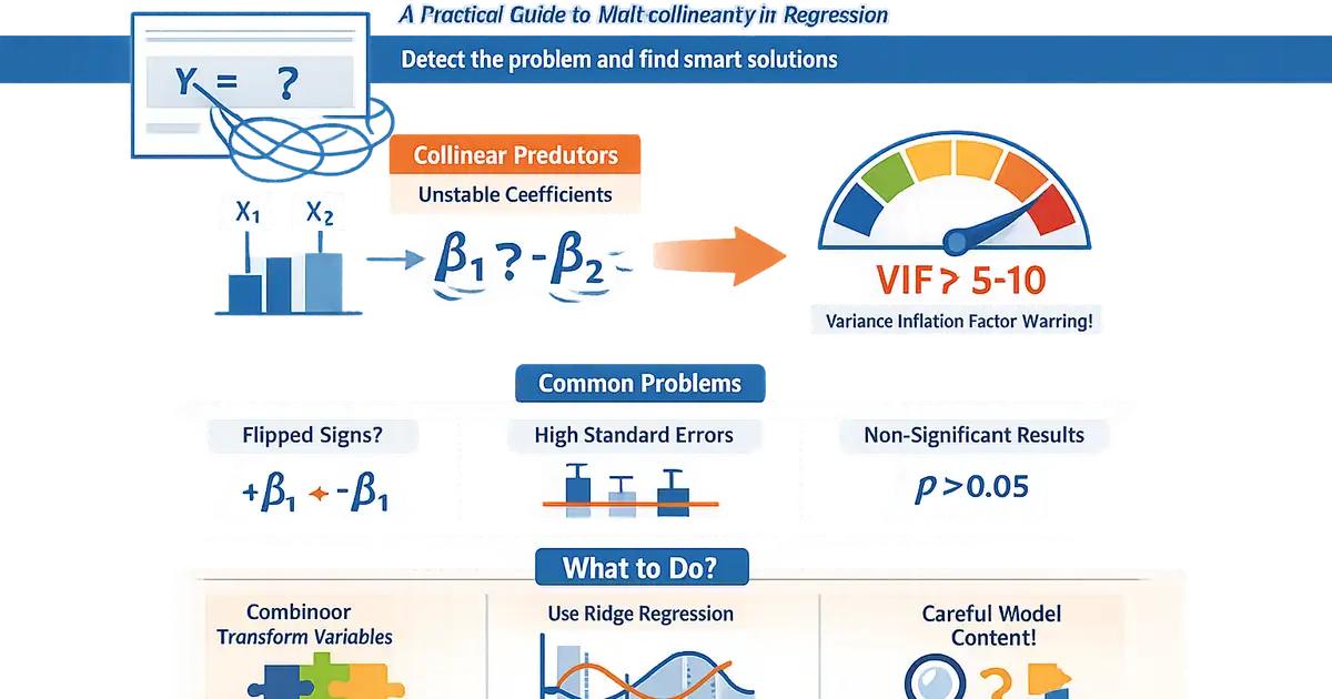
A practical guide to multicollinearity in regression. Learn when collinearity is a problem, how to detect it, and practical solutions that don't involve blindly dropping variables.
Quick Hits
- •Collinearity = correlated predictors → unstable coefficient estimates
- •VIF > 5-10 signals potential problems (but context matters)
- •Coefficients may flip sign or become non-significant - not because of bad data, but because they're poorly identified
- •Perfect collinearity is detectable (model fails); high collinearity is harder
- •Solutions depend on your goal: prediction doesn't care, interpretation does
TL;DR
Multicollinearity occurs when predictor variables are highly correlated. It doesn't bias coefficients, but it inflates standard errors, making individual predictors hard to interpret. VIF > 5-10 signals problems. Solutions include combining variables, ridge regression, or simply accepting that correlated effects can't be separated. The key insight: collinearity is a problem for interpretation, not prediction.
What Is Collinearity?
Definition
Multicollinearity occurs when predictor variables in a regression model are correlated with each other. This creates problems because the model can't distinguish the individual effects.
Perfect Collinearity
If one predictor is a perfect linear function of others:
- X₃ = 2X₁ + 5X₂
The model cannot be fit. Software will drop a variable or throw an error.
Common cause: Including a dummy variable for all categories (the "dummy variable trap").
High Collinearity
More common and more insidious: predictors are highly but not perfectly correlated.
- Age and years of experience
- Revenue and customer count
- Multiple survey items measuring the same construct
Why Collinearity Is a Problem
The Core Issue
When X₁ and X₂ are highly correlated, the model can't tell which one is "responsible" for the effect.
Extreme example: X₁ and X₂ are nearly identical
- Model could attribute the effect to X₁ and not X₂
- Or to X₂ and not X₁
- Or split between them in any way
What Happens to Estimates
| Aspect | Effect of Collinearity |
|---|---|
| Coefficient estimates | Unbiased (still correct on average) |
| Standard errors | Inflated (often dramatically) |
| t-statistics | Reduced (harder to find significance) |
| Coefficient stability | Unstable (small data changes → big coefficient changes) |
| Signs | May flip (positive becomes negative) |
| Overall R² | Usually unaffected |
| Predictions | Usually unaffected |
The Paradox
You might see:
- High overall R² (model explains a lot)
- None of the individual coefficients significant
- Coefficients with "wrong" signs
This isn't a contradiction—the predictors together explain the outcome, but the model can't attribute credit to individuals.
Detecting Collinearity
Method 1: Correlation Matrix
Look for high pairwise correlations (r > 0.7-0.8).
Limitation: Misses multiway collinearity (X₃ is a linear combination of X₁ and X₂, even if no pair is highly correlated).
Method 2: Variance Inflation Factor (VIF)
VIF measures how much the variance of a coefficient is inflated due to collinearity.
Where is the R² from regressing predictor on all other predictors.
Interpretation:
- VIF = 1: No collinearity
- VIF = 5: Variance is 5× what it would be without collinearity
- VIF = 10: Standard error is larger
Thresholds (rules of thumb):
- VIF > 5: Moderate concern
- VIF > 10: Serious concern
- VIF > 100: Near-perfect collinearity
Method 3: Condition Number
The condition number of the predictor matrix is another diagnostic.
-
30: Serious collinearity
Method 4: Symptoms
Watch for these signs:
- Coefficients change dramatically when adding/removing variables
- Coefficients have opposite signs from bivariate correlations
- High R² but no significant individual predictors
- Very large standard errors
Code: Detecting Collinearity
Python
import numpy as np
import pandas as pd
import statsmodels.api as sm
import statsmodels.formula.api as smf
from statsmodels.stats.outliers_influence import variance_inflation_factor


def check_collinearity(model):
    """
    Comprehensive collinearity diagnostics.

    Parameters:
    -----------
    model : statsmodels RegressionResults
        Fitted OLS model

    Returns:
    --------
    dict with diagnostics
    """
    results = {}

    # Get predictor matrix (excluding intercept for VIF)
    X = model.model.exog
    feature_names = model.model.exog_names

    # Correlation matrix (excluding intercept)
    if 'Intercept' in feature_names or 'const' in feature_names:
        X_no_const = X[:, 1:]
        names_no_const = [n for n in feature_names if n not in ['Intercept', 'const']]
    else:
        X_no_const = X
        names_no_const = feature_names

    corr_matrix = pd.DataFrame(
        np.corrcoef(X_no_const.T),
        columns=names_no_const,
        index=names_no_const
    )
    results['correlation_matrix'] = corr_matrix

    # High correlations
    high_corr = []
    for i, var1 in enumerate(names_no_const):
        for j, var2 in enumerate(names_no_const):
            if i < j and abs(corr_matrix.iloc[i, j]) > 0.7:
                high_corr.append({
                    'var1': var1,
                    'var2': var2,
                    'correlation': corr_matrix.iloc[i, j]
                })
    results['high_correlations'] = pd.DataFrame(high_corr)

    # VIF
    vif_data = []
    for i, name in enumerate(feature_names):
        vif = variance_inflation_factor(X, i)
        vif_data.append({'Variable': name, 'VIF': vif})

    vif_df = pd.DataFrame(vif_data)
    results['vif'] = vif_df

    # Flag problematic variables
    results['high_vif_variables'] = vif_df[vif_df['VIF'] > 5]['Variable'].tolist()
    if 'Intercept' in results['high_vif_variables']:
        results['high_vif_variables'].remove('Intercept')
    if 'const' in results['high_vif_variables']:
        results['high_vif_variables'].remove('const')

    # Condition number
    results['condition_number'] = np.linalg.cond(X)

    # Summary flags
    results['has_collinearity_issues'] = (
        len(results['high_vif_variables']) > 0 or
        results['condition_number'] > 30
    )

    return results


def compare_coefficient_stability(data, formula, drop_vars):
    """
    Check how coefficients change when dropping variables.

    Helps identify which variables are causing instability.
    """
    # Full model
    full_model = smf.ols(formula, data=data).fit()

    comparisons = [{'Model': 'Full', **dict(zip(full_model.params.index, full_model.params.values))}]

    # Models dropping each variable
    for var in drop_vars:
        reduced_formula = formula.replace(f' + {var}', '').replace(f'{var} + ', '')
        if var in reduced_formula:
            reduced_formula = reduced_formula.replace(var, '').replace(' ~ +', ' ~').replace('+ +', '+')

        try:
            reduced_model = smf.ols(reduced_formula, data=data).fit()
            row = {'Model': f'Drop {var}'}
            for param in full_model.params.index:
                if param in reduced_model.params.index:
                    row[param] = reduced_model.params[param]
                else:
                    row[param] = np.nan
            comparisons.append(row)
        except:
            pass

    return pd.DataFrame(comparisons)


# Example
if __name__ == "__main__":
    np.random.seed(42)
    n = 200

    # Create data with collinearity
    x1 = np.random.normal(0, 1, n)
    x2 = x1 + np.random.normal(0, 0.3, n)  # Highly correlated with x1
    x3 = np.random.normal(0, 1, n)  # Independent

    y = 2 + 3*x1 + 2*x2 + 1*x3 + np.random.normal(0, 1, n)

    data = pd.DataFrame({'y': y, 'x1': x1, 'x2': x2, 'x3': x3})

    # Fit model
    model = smf.ols('y ~ x1 + x2 + x3', data=data).fit()

    print("Model Summary")
    print("=" * 50)
    print(model.summary().tables[1])

    print("\n" + "=" * 50)
    print("Collinearity Diagnostics")
    diagnostics = check_collinearity(model)

    print("\nVIF:")
    print(diagnostics['vif'].to_string(index=False))

    print(f"\nCondition Number: {diagnostics['condition_number']:.1f}")
    print(f"\nHigh VIF Variables: {diagnostics['high_vif_variables']}")

    if len(diagnostics['high_correlations']) > 0:
        print("\nHigh Correlations:")
        print(diagnostics['high_correlations'].to_string(index=False))
R
library(tidyverse)
library(car)  # For VIF


check_collinearity <- function(model) {
    #' Comprehensive collinearity diagnostics

    # VIF
    vif_values <- vif(model)
    vif_df <- tibble(
        Variable = names(vif_values),
        VIF = as.numeric(vif_values)
    )

    # Correlation matrix of predictors
    X <- model.matrix(model)[, -1]  # Exclude intercept
    corr_matrix <- cor(X)

    # Find high correlations
    high_corr <- which(abs(corr_matrix) > 0.7 & corr_matrix != 1, arr.ind = TRUE)
    high_corr_pairs <- if (nrow(high_corr) > 0) {
        data.frame(
            var1 = rownames(corr_matrix)[high_corr[, 1]],
            var2 = colnames(corr_matrix)[high_corr[, 2]],
            correlation = corr_matrix[high_corr]
        ) %>%
            filter(as.character(var1) < as.character(var2))
    } else {
        data.frame(var1 = character(), var2 = character(), correlation = numeric())
    }

    # Condition number
    condition_num <- kappa(X, exact = TRUE)

    list(
        vif = vif_df,
        correlation_matrix = corr_matrix,
        high_correlations = high_corr_pairs,
        condition_number = condition_num,
        high_vif_variables = vif_df$Variable[vif_df$VIF > 5],
        has_issues = any(vif_df$VIF > 5) | condition_num > 30
    )
}


# Example
set.seed(42)
n <- 200

data <- tibble(
    x1 = rnorm(n),
    x2 = x1 + rnorm(n, 0, 0.3),  # Correlated with x1
    x3 = rnorm(n)
) %>%
    mutate(y = 2 + 3*x1 + 2*x2 + 1*x3 + rnorm(n))

model <- lm(y ~ x1 + x2 + x3, data = data)

cat("Model Summary\n")
cat(strrep("=", 50), "\n")
print(summary(model))

cat("\nCollinearity Diagnostics\n")
cat(strrep("=", 50), "\n")
diagnostics <- check_collinearity(model)
cat("\nVIF:\n")
print(diagnostics$vif)
cat(sprintf("\nCondition Number: %.1f\n", diagnostics$condition_number))
cat(sprintf("High VIF Variables: %s\n", paste(diagnostics$high_vif_variables, collapse = ", ")))
Solutions for Collinearity
Solution 1: Do Nothing (Seriously)
When appropriate:
- Your goal is prediction, not coefficient interpretation
- The collinear variables are controls, not your focus
- You accept that these effects can't be separated
Why it's valid: Predictions are still good; R² is unaffected.
Solution 2: Combine Variables
If X₁ and X₂ measure the same underlying thing, combine them:
# Average
data['combined'] = (data['x1'] + data['x2']) / 2

# PCA
from sklearn.decomposition import PCA
pca = PCA(n_components=1)
data['pc1'] = pca.fit_transform(data[['x1', 'x2']])

# Factor analysis
# If you have multiple indicators of the same construct
When appropriate:
- Variables conceptually measure the same thing
- You don't need to separate their effects
Solution 3: Drop One Variable
When appropriate:
- One variable is clearly redundant
- You have strong theoretical reason to prefer one
- Sensitivity analysis shows results are robust
Caution: Dropping a variable that belongs in the model creates omitted variable bias. Don't drop just because of high VIF.
Solution 4: Ridge Regression
Ridge regression adds a penalty that shrinks coefficients, stabilizing them under collinearity.
from sklearn.linear_model import Ridge, RidgeCV

# Cross-validated ridge
ridge_cv = RidgeCV(alphas=[0.01, 0.1, 1, 10, 100])
ridge_cv.fit(X, y)

print(f"Best alpha: {ridge_cv.alpha_}")
print(f"Coefficients: {ridge_cv.coef_}")
Trade-off: Coefficients are biased toward zero but more stable. Predictions often improve.
Solution 5: Get More Data
More data reduces variance of all estimates, partially mitigating collinearity issues.
Limitation: Doesn't help if collinearity is inherent (age and experience will always correlate).
Solution 6: Center Predictors
Centering reduces collinearity involving interactions:
data['x1_centered'] = data['x1'] - data['x1'].mean()
data['x2_centered'] = data['x2'] - data['x2'].mean()
Limitation: Only helps with certain types of collinearity (especially with polynomial/interaction terms).
Solution Decision Framework
START: High VIF or collinearity detected
       ↓
QUESTION: Is your goal prediction or interpretation?
├── Prediction → Likely OK to proceed (check prediction accuracy)
└── Interpretation → Continue
       ↓
QUESTION: Are collinear variables your focus or controls?
├── Controls → Likely OK if main variables are fine
└── Focus variables → Continue
       ↓
QUESTION: Do collinear variables measure the same construct?
├── Yes → Combine them (average, PCA, factor analysis)
└── No → Continue
       ↓
QUESTION: Is one variable clearly more important theoretically?
├── Yes → Consider dropping the other (with sensitivity check)
└── No → Continue
       ↓
CONSIDER:
- Ridge regression (biased but stable)
- Accept that effects can't be separated
- Report partial effects and total effect of combined variables
When Collinearity Isn't a Problem
For Prediction
Collinearity doesn't hurt prediction. If your goal is forecasting or risk scoring, high VIF may not matter.
For Categorical Variables
Dummy variables for a categorical variable will be correlated (choosing Category B means not choosing Category A). This is fine—VIF among dummies is expected.
Don't drop dummies to reduce VIF—that changes your reference category interpretation.
For Interaction Terms
Main effects and interactions are often correlated. This is expected:
x1, x2, x1*x2 → VIF will be high for interaction
Solution: Center the main effects before creating interactions. Reduces VIF without changing interpretation.
For Polynomial Terms
x and x² are correlated by construction.
Solution: Use orthogonal polynomials or center x before squaring.
Common Mistakes
Mistake 1: Automatically Dropping High-VIF Variables
Wrong: "VIF > 10, so I dropped x2"
Problem: If x2 belongs in the model, dropping it creates omitted variable bias. Now your other coefficients are wrong.
Better: Consider why these variables are correlated and whether you need to separate them.
Mistake 2: Using VIF Threshold Blindly
Wrong: "All VIFs are below 10, so no collinearity problem"
Problem: VIF thresholds are arbitrary. VIF = 9 might still cause issues; VIF = 12 might be acceptable for control variables.
Better: Consider the context and your interpretive goals.
Mistake 3: Ignoring Collinearity When Interpreting
Wrong: "The coefficient on x1 is 5 and significant"
Problem: If x1 and x2 are collinear, the coefficient on x1 is conditional on holding x2 constant—but x1 and x2 move together in reality.
Better: Acknowledge that these effects can't be cleanly separated.
Mistake 4: Blaming Collinearity for Everything
Wrong: "Results don't make sense—must be collinearity"
Reality: Collinearity causes high variance, not bias. If coefficients have wrong signs, it might be:
- Normal variance (check CIs—do they include "correct" values?)
- Model misspecification
- Confounding
Related Methods
- Regression for Analysts (Pillar) - Complete regression framework
- Linear Regression Diagnostics - Other diagnostics
- Feature Scaling and Transforms - Centering to reduce collinearity
- Interaction Terms - Managing interaction collinearity
Key Takeaway
Collinearity makes individual coefficients hard to interpret because correlated predictors "share credit" for explaining the outcome. Coefficients become unstable with inflated standard errors, but predictions remain valid. Before dropping variables (which risks omitted variable bias), consider whether you truly need to separate these effects. Combining variables, ridge regression, or simply acknowledging the limitation may be better than creating new problems by dropping important predictors.
References
- https://www.jstor.org/stable/2685573
- https://journalofbigdata.springeropen.com/articles/10.1186/s40537-019-0252-9
- https://online.stat.psu.edu/stat462/node/177/
- Belsley, D. A., Kuh, E., & Welsch, R. E. (1980). Regression diagnostics: Identifying influential data and sources of collinearity. Wiley.
- O'Brien, R. M. (2007). A caution regarding rules of thumb for variance inflation factors. *Quality & Quantity*, 41(5), 673-690.
- Penn State STAT 462. Lesson 12: Multicollinearity. Online course materials.
Frequently Asked Questions
Does collinearity bias my coefficient estimates?
What VIF threshold should I use?
Should I just drop the correlated variable?
Key Takeaway
Collinearity makes individual coefficients hard to interpret, but overall predictions may still be fine. Check VIF, but don't blindly drop variables—that can introduce bias. Consider whether you truly need to separate the correlated effects, or whether a combined measure or dimension reduction makes more sense.