Contents
Linear Regression Assumptions and Diagnostics in Practice
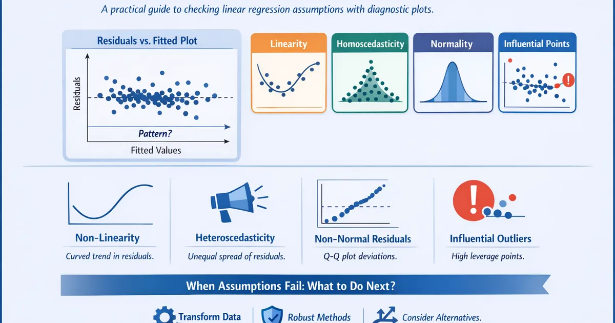
A practical guide to checking linear regression assumptions with diagnostic plots. Learn what violations actually look like, when they matter, and what to do when assumptions fail.
Quick Hits
- •Linearity and homoscedasticity violations are serious - they bias coefficients or standard errors
- •Normality violations are often minor - especially with large samples
- •Independence is the hardest to check and most damaging when violated
- •One influential point can completely change your conclusions
- •Always plot residuals vs. fitted before interpreting any regression
TL;DR
Linear regression makes assumptions about your data. When assumptions hold, coefficients are unbiased and standard errors are correct. When they fail, you may have wrong answers and misleading p-values. This guide shows you how to diagnose violations using residual plots, explains when violations actually matter, and provides practical fixes. The key insight: always check residuals vs. fitted before trusting your results.
The Four Core Assumptions
Linear regression assumes:
- Linearity: The relationship between predictors and outcome is linear
- Independence: Observations are independent of each other
- Homoscedasticity: Variance of residuals is constant across fitted values
- Normality: Residuals are normally distributed
Memory device: LINE (Linearity, Independence, Normality, Equal variance)
What Happens When Assumptions Fail
| Assumption | Violation Effect | Consequence |
|---|---|---|
| Linearity | Biased coefficients | Wrong conclusions about relationships |
| Independence | Understated standard errors | Too many false positives |
| Homoscedasticity | Inefficient estimates, wrong SEs | Unreliable confidence intervals |
| Normality | Unreliable p-values and CIs | (Minor with large n) |
Diagnostic Plot 1: Residuals vs. Fitted
What it shows: Linearity and homoscedasticity
What to look for:
- Random scatter around zero = good
- Curved pattern = non-linearity
- Funnel shape = heteroscedasticity
Good Pattern
     |    *     *
     |  *   *  *   *
  0 -|--*--*--*--*--*--
     |    * *   *
     |  *    *     *
     +------------------
       Fitted Values
Random scatter, no pattern, consistent spread.
Bad: Non-Linearity
     |           ***
     |        ***
  0 -|------*------
     |   ***
     |***
     +------------------
       Fitted Values
Curved pattern indicates missing quadratic or other non-linear terms.
Bad: Heteroscedasticity
     |               *
     |             * * *
  0 -|-*-*-*----*---*---
     |  * *    *  *
     |          *   *
     +------------------
       Fitted Values
Fan shape: variance increases with fitted values.
Diagnostic Plot 2: Q-Q Plot
What it shows: Normality of residuals
What to look for:
- Points following the diagonal line = normal
- S-shape = heavy tails
- Curved away from line at one end = skewness
Good Pattern
Points lie approximately on the diagonal line, with perhaps minor deviations at the tails.
Bad: Heavy Tails
     +
    +  |
   +   |
  +    |
 +     | <- Points above line at right
       |
       | <- Points below line at left
More extreme values than normal distribution predicts.
Bad: Skewness
       |     ++++++
       |   ++
       | ++
       |+
      +|
    ++ |
  ++   |
Asymmetric distribution of residuals.
Diagnostic Plot 3: Scale-Location
What it shows: Homoscedasticity (same as residuals vs. fitted, different view)
Plots: vs. Fitted Values
What to look for:
- Horizontal band = constant variance
- Upward trend = variance increases with fitted values
- Downward trend = variance decreases with fitted values
Diagnostic Plot 4: Residuals vs. Leverage
What it shows: Influential observations
Key concepts:
- Leverage: How unusual is an observation's predictor values?
- Residual: How far is the observation from the prediction?
- Cook's Distance: Combined influence (leverage × residual)
What to look for:
- High leverage + high residual = problematic
- Points beyond Cook's distance contours (usually 0.5 or 1) need investigation
Code: Complete Diagnostic Workflow
Python
import numpy as np
import pandas as pd
import statsmodels.api as sm
import statsmodels.formula.api as smf
from statsmodels.stats.diagnostic import het_breuschpagan, linear_rainbow
from statsmodels.stats.stattools import durbin_watson
from scipy import stats
import matplotlib.pyplot as plt


def comprehensive_diagnostics(model, data, figsize=(14, 12)):
    """
    Run complete regression diagnostics.

    Parameters:
    -----------
    model : statsmodels RegressionResults
        Fitted OLS model
    data : pd.DataFrame
        Original data

    Returns:
    --------
    dict with diagnostic results and flags
    """
    n = len(model.resid)

    # Extract diagnostic quantities
    fitted = model.fittedvalues
    residuals = model.resid
    influence = model.get_influence()
    standardized_resid = influence.resid_studentized_internal
    leverage = influence.hat_matrix_diag
    cooks_d = influence.cooks_distance[0]

    # Statistical tests
    diagnostics = {}

    # 1. Linearity (Rainbow test)
    try:
        rainbow_stat, rainbow_p = linear_rainbow(model)
        diagnostics['linearity'] = {
            'test': 'Rainbow',
            'statistic': rainbow_stat,
            'p_value': rainbow_p,
            'flag': rainbow_p < 0.05
        }
    except:
        diagnostics['linearity'] = {'test': 'Rainbow', 'error': 'Could not compute'}

    # 2. Homoscedasticity (Breusch-Pagan)
    bp_stat, bp_p, _, _ = het_breuschpagan(residuals, model.model.exog)
    diagnostics['homoscedasticity'] = {
        'test': 'Breusch-Pagan',
        'statistic': bp_stat,
        'p_value': bp_p,
        'flag': bp_p < 0.05
    }

    # 3. Normality (Shapiro-Wilk, sample if n > 5000)
    resid_sample = residuals if n <= 5000 else np.random.choice(residuals, 5000)
    shapiro_stat, shapiro_p = stats.shapiro(resid_sample)
    diagnostics['normality'] = {
        'test': 'Shapiro-Wilk',
        'statistic': shapiro_stat,
        'p_value': shapiro_p,
        'flag': shapiro_p < 0.05
    }

    # 4. Independence (Durbin-Watson for autocorrelation)
    dw_stat = durbin_watson(residuals)
    diagnostics['independence'] = {
        'test': 'Durbin-Watson',
        'statistic': dw_stat,
        'interpretation': 'Positive autocorr' if dw_stat < 1.5 else (
            'Negative autocorr' if dw_stat > 2.5 else 'No autocorr'),
        'flag': dw_stat < 1.5 or dw_stat > 2.5
    }

    # 5. Influential points
    high_leverage_threshold = 2 * (model.df_model + 1) / n
    high_leverage = np.sum(leverage > high_leverage_threshold)
    high_cooks = np.sum(cooks_d > 4/n)

    diagnostics['influential_points'] = {
        'high_leverage_count': high_leverage,
        'high_cooks_count': high_cooks,
        'max_cooks_d': np.max(cooks_d),
        'flag': high_cooks > 0
    }

    # Create diagnostic plots
    fig, axes = plt.subplots(2, 2, figsize=figsize)

    # Plot 1: Residuals vs Fitted
    ax1 = axes[0, 0]
    ax1.scatter(fitted, residuals, alpha=0.6, edgecolors='none')
    ax1.axhline(y=0, color='red', linestyle='--', linewidth=1)
    # Lowess smoothing
    from statsmodels.nonparametric.smoothers_lowess import lowess
    smooth = lowess(residuals, fitted, frac=0.3)
    ax1.plot(smooth[:, 0], smooth[:, 1], 'r-', linewidth=2, label='Lowess')
    ax1.set_xlabel('Fitted Values')
    ax1.set_ylabel('Residuals')
    ax1.set_title('Residuals vs Fitted\n(Check: Linearity, Homoscedasticity)')

    # Plot 2: Q-Q Plot
    ax2 = axes[0, 1]
    stats.probplot(standardized_resid, dist="norm", plot=ax2)
    ax2.set_title('Normal Q-Q\n(Check: Normality)')
    ax2.get_lines()[0].set_markerfacecolor('steelblue')
    ax2.get_lines()[0].set_alpha(0.6)

    # Plot 3: Scale-Location
    ax3 = axes[1, 0]
    sqrt_std_resid = np.sqrt(np.abs(standardized_resid))
    ax3.scatter(fitted, sqrt_std_resid, alpha=0.6, edgecolors='none')
    smooth = lowess(sqrt_std_resid, fitted, frac=0.3)
    ax3.plot(smooth[:, 0], smooth[:, 1], 'r-', linewidth=2)
    ax3.set_xlabel('Fitted Values')
    ax3.set_ylabel('√|Standardized Residuals|')
    ax3.set_title('Scale-Location\n(Check: Homoscedasticity)')

    # Plot 4: Residuals vs Leverage
    ax4 = axes[1, 1]
    ax4.scatter(leverage, standardized_resid, alpha=0.6, edgecolors='none')
    ax4.axhline(y=0, color='grey', linestyle='--', linewidth=0.5)

    # Cook's distance contours
    xlim = ax4.get_xlim()
    x_vals = np.linspace(0.001, xlim[1], 100)
    for thresh in [0.5, 1.0]:
        y_vals = np.sqrt(thresh * n * (1 - x_vals) / x_vals / model.df_model)
        ax4.plot(x_vals, y_vals, 'r--', linewidth=0.5, alpha=0.7)
        ax4.plot(x_vals, -y_vals, 'r--', linewidth=0.5, alpha=0.7)

    ax4.set_xlabel('Leverage')
    ax4.set_ylabel('Standardized Residuals')
    ax4.set_title('Residuals vs Leverage\n(Check: Influential Points)')

    # Annotate highly influential points
    for i, (lev, resid, cd) in enumerate(zip(leverage, standardized_resid, cooks_d)):
        if cd > 4/n:
            ax4.annotate(str(i), (lev, resid), fontsize=8)

    plt.tight_layout()

    # Summary
    flags = []
    if diagnostics['linearity'].get('flag'):
        flags.append("⚠️ Non-linearity detected (Rainbow test p < 0.05)")
    if diagnostics['homoscedasticity']['flag']:
        flags.append("⚠️ Heteroscedasticity detected (Breusch-Pagan p < 0.05)")
    if diagnostics['normality']['flag']:
        flags.append("⚠️ Non-normality detected (Shapiro-Wilk p < 0.05)")
    if diagnostics['independence']['flag']:
        flags.append(f"⚠️ Autocorrelation detected (DW = {dw_stat:.2f})")
    if diagnostics['influential_points']['flag']:
        flags.append(f"⚠️ {high_cooks} influential point(s) (Cook's d > 4/n)")

    return {
        'diagnostics': diagnostics,
        'flags': flags,
        'figure': fig
    }


# Example usage
if __name__ == "__main__":
    np.random.seed(42)
    n = 200

    # Create data with some issues
    x1 = np.random.normal(0, 1, n)
    x2 = np.random.uniform(0, 10, n)

    # Non-linear relationship (quadratic)
    y = 2 + 3*x1 + 0.5*x2 - 0.2*x1**2 + np.random.normal(0, 1, n)

    data = pd.DataFrame({'y': y, 'x1': x1, 'x2': x2})

    # Fit linear model (missing quadratic term)
    model = smf.ols('y ~ x1 + x2', data=data).fit()

    # Run diagnostics
    results = comprehensive_diagnostics(model, data)

    print("Diagnostic Summary")
    print("=" * 50)
    for flag in results['flags']:
        print(flag)
    if not results['flags']:
        print("✓ No major assumption violations detected")

    plt.show()
R
library(tidyverse)
library(broom)
library(car)
library(lmtest)


comprehensive_diagnostics <- function(model) {
    #' Run complete regression diagnostics

    n <- length(residuals(model))
    p <- length(coef(model))

    # Calculate diagnostic quantities
    resids <- residuals(model)
    std_resids <- rstandard(model)
    fitted_vals <- fitted(model)
    leverage <- hatvalues(model)
    cooks <- cooks.distance(model)

    # Statistical tests
    results <- list()

    # 1. Linearity (Rainbow test)
    rainbow_test <- tryCatch({
        lmtest::raintest(model)
    }, error = function(e) NULL)

    if (!is.null(rainbow_test)) {
        results$linearity <- list(
            test = "Rainbow",
            statistic = rainbow_test$statistic,
            p_value = rainbow_test$p.value,
            flag = rainbow_test$p.value < 0.05
        )
    }

    # 2. Homoscedasticity (Breusch-Pagan)
    bp_test <- lmtest::bptest(model)
    results$homoscedasticity <- list(
        test = "Breusch-Pagan",
        statistic = bp_test$statistic,
        p_value = bp_test$p.value,
        flag = bp_test$p.value < 0.05
    )

    # 3. Normality (Shapiro-Wilk)
    resid_sample <- if (n > 5000) sample(resids, 5000) else resids
    sw_test <- shapiro.test(resid_sample)
    results$normality <- list(
        test = "Shapiro-Wilk",
        statistic = sw_test$statistic,
        p_value = sw_test$p.value,
        flag = sw_test$p.value < 0.05
    )

    # 4. Independence (Durbin-Watson)
    dw_test <- lmtest::dwtest(model)
    results$independence <- list(
        test = "Durbin-Watson",
        statistic = dw_test$statistic,
        p_value = dw_test$p.value,
        flag = dw_test$p.value < 0.05
    )

    # 5. Influential points
    high_leverage_thresh <- 2 * p / n
    results$influential <- list(
        high_leverage_count = sum(leverage > high_leverage_thresh),
        high_cooks_count = sum(cooks > 4/n),
        max_cooks = max(cooks),
        flag = sum(cooks > 4/n) > 0
    )

    # Generate flags
    flags <- c()
    if (results$linearity$flag) {
        flags <- c(flags, "⚠️ Non-linearity detected (Rainbow test)")
    }
    if (results$homoscedasticity$flag) {
        flags <- c(flags, "⚠️ Heteroscedasticity detected (Breusch-Pagan)")
    }
    if (results$normality$flag) {
        flags <- c(flags, "⚠️ Non-normality detected (Shapiro-Wilk)")
    }
    if (results$independence$flag) {
        flags <- c(flags, "⚠️ Autocorrelation detected (Durbin-Watson)")
    }
    if (results$influential$flag) {
        flags <- c(flags, sprintf("⚠️ %d influential point(s) detected",
                                  results$influential$high_cooks_count))
    }

    list(
        tests = results,
        flags = flags
    )
}


plot_diagnostics_enhanced <- function(model) {
    #' Create enhanced diagnostic plots

    par(mfrow = c(2, 2))

    # Standard plots with better formatting
    plot(model, which = 1, main = "Residuals vs Fitted\n(Check: Linearity, Homoscedasticity)")
    plot(model, which = 2, main = "Normal Q-Q\n(Check: Normality)")
    plot(model, which = 3, main = "Scale-Location\n(Check: Homoscedasticity)")
    plot(model, which = 5, main = "Residuals vs Leverage\n(Check: Influential Points)")

    par(mfrow = c(1, 1))
}


# Example usage
set.seed(42)
n <- 200

data <- tibble(
    x1 = rnorm(n),
    x2 = runif(n, 0, 10)
) %>%
    mutate(y = 2 + 3*x1 + 0.5*x2 - 0.2*x1^2 + rnorm(n))

# Fit model (missing quadratic)
model <- lm(y ~ x1 + x2, data = data)

# Run diagnostics
results <- comprehensive_diagnostics(model)

cat("Diagnostic Summary\n")
cat(strrep("=", 50), "\n")
if (length(results$flags) > 0) {
    for (flag in results$flags) {
        cat(flag, "\n")
    }
} else {
    cat("✓ No major assumption violations detected\n")
}

# Plot
plot_diagnostics_enhanced(model)
What To Do When Assumptions Fail
Non-Linearity Detected
Options:
- Add polynomial terms:
y ~ x + I(x^2) - Add interaction terms:
y ~ x1 * x2 - Transform predictors:
y ~ log(x) - Use splines or GAMs for flexible non-linearity
# Adding polynomial term
model_quad = smf.ols('y ~ x1 + I(x1**2) + x2', data=data).fit()
Heteroscedasticity Detected
Options:
- Use robust standard errors (doesn't fix inefficiency, does fix SEs)
- Transform the outcome (log transformation common for positive data)
- Use weighted least squares
- Use a generalized linear model with appropriate variance function
# Robust standard errors
from statsmodels.stats.sandwich_covariance import cov_hc3
robust_cov = cov_hc3(model)
robust_se = np.sqrt(np.diag(robust_cov))
Non-Normality Detected
When to worry:
- Small samples (n < 50): May affect CI coverage
- Large samples: Usually fine (CLT)
- Severe skewness: Consider transformation
Options:
- Transform outcome (log, sqrt, Box-Cox)
- Use robust regression (M-estimators)
- Bootstrap for inference
- With large n, often acceptable to proceed
Independence Violated
This is serious. Standard errors are wrong, often too small.
Options:
- Clustered standard errors (cluster at the level of dependency)
- Mixed effects models (for hierarchical data)
- Time series models (for autocorrelated data)
- GEE for repeated measures
# Clustered standard errors
library(sandwich)
library(lmtest)
coeftest(model, vcov = vcovCL(model, cluster = ~group_id))
Influential Points Detected
Steps:
- Identify which observations (check Cook's distance)
- Investigate: Are they data errors? Valid outliers?
- Run analysis with and without them
- Report both results if conclusions differ
- Consider robust regression if outliers are valid but influential
Practical Guidelines: When Violations Matter
Rules of Thumb
| Violation | When It's Serious | When It's Often OK |
|---|---|---|
| Non-linearity | Always problematic | Never OK to ignore |
| Independence | Always problematic | Never OK to ignore |
| Heteroscedasticity | Small samples, prediction intervals | Large samples with robust SEs |
| Non-normality | Small samples (<30) | Large samples, moderate deviations |
Sample Size Buffer
With larger samples, some violations matter less:
- n > 30: Moderate non-normality usually OK
- n > 100: More robust to most violations
- n > 500: Focus mainly on linearity and independence
Effect on Different Quantities
| Quantity | Most Affected By |
|---|---|
| Coefficient estimates | Non-linearity, influential points |
| Standard errors | Heteroscedasticity, independence |
| P-values | All violations (via SEs) |
| Prediction intervals | Heteroscedasticity, non-normality |
| R² | Non-linearity |
The Diagnostic Decision Tree
START: Fit your model

↓

CHECK: Residuals vs Fitted
├── Curved pattern? → Add polynomial terms or transform
├── Funnel shape? → Use robust SEs or transform outcome
└── Random scatter? → Continue

↓

CHECK: Q-Q Plot
├── Severe deviations? + Small sample → Consider transformation
├── Moderate deviations? + Large sample → Usually proceed
└── Points on line? → Continue

↓

CHECK: Leverage/Cook's D
├── High influence points? → Investigate, run sensitivity analysis
└── No issues? → Continue

↓

CHECK: Data structure
├── Clustered/hierarchical? → Use clustered SEs or mixed models
├── Time series? → Check Durbin-Watson, consider time series model
└── Independent? → Continue

↓

PROCEED with interpretation
Related Methods
- Regression for Analysts (Pillar) - Complete regression framework
- Robust Standard Errors - Fixing heteroscedasticity
- Handling Outliers - Robust alternatives
- Transformations Guide - When transforms help
Key Takeaway
Diagnostic plots are more important than the regression output itself. A significant coefficient is meaningless if assumptions are violated and standard errors are wrong. Always check residuals vs. fitted (for linearity and homoscedasticity), Q-Q plots (for normality), and Cook's distance (for influential points). When violations occur, the fix depends on which assumption failed—robust standard errors for heteroscedasticity, polynomials for non-linearity, mixed models for clustering. Never skip diagnostics.
References
- https://www.stat.berkeley.edu/~aldous/157/Papers/Fox.pdf
- https://data.library.virginia.edu/diagnostic-plots/
- https://onlinelibrary.wiley.com/doi/10.1002/sim.3782
- Fox, J. (2015). Applied regression analysis and generalized linear models. Sage Publications.
- University of Virginia Library. Diagnostic plots in R. Research Data Services.
- Williams, M. N., Grajales, C. A. G., & Kurkiewicz, D. (2013). Assumptions of multiple regression. *International Journal of Research & Method in Education*, 36(2), 164-185.
Frequently Asked Questions
Which assumption is most important?
Can I use regression if my data isn't normal?
What's the difference between residual plots and looking at raw data distributions?
Key Takeaway
Regression diagnostics are about checking whether your model captures the systematic patterns in your data and whether your uncertainty estimates are trustworthy. Always plot residuals vs. fitted values first - most problems show up there.