Contents
Handling Outliers: Trimmed Means, Winsorization, and Robust Methods
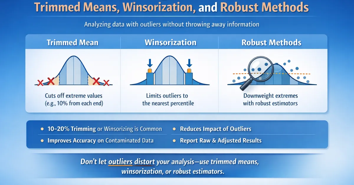
How to analyze data with outliers without throwing away information or letting extreme values dominate. Covers trimming, winsorization, robust estimators, and when each is appropriate.
Quick Hits
- •Trimming removes extreme values; winsorization caps them at percentiles
- •10-20% trimming (each tail) is common; decide before seeing data
- •Robust methods often perform as well as standard methods on clean data and much better on contaminated data
- •Document your outlier handling and report both raw and adjusted results
TL;DR
Outliers can dominate means and inflate variance, making your analysis misleading. Principled solutions include trimmed means (removing a fixed percentage from each tail), winsorization (capping extremes at percentiles), and robust estimators (downweighting outliers automatically). Choose your method before seeing data and be clear about what you're estimating.
The Problem with Outliers
A single extreme value can:
- Shift the sample mean dramatically
- Inflate variance estimates
- Reduce statistical power
- Mask real effects or create spurious ones
import numpy as np
from scipy import stats

# Clean data: treatment is clearly better
clean_control = np.random.normal(100, 10, 50)
clean_treatment = np.random.normal(105, 10, 50)  # 5 unit lift

stat, p_clean = stats.ttest_ind(clean_control, clean_treatment)
print(f"Clean data: diff = {np.mean(clean_treatment) - np.mean(clean_control):.1f}, p = {p_clean:.4f}")

# Add one outlier to treatment
contaminated_treatment = np.append(clean_treatment[:-1], 500)  # One extreme value

stat, p_contaminated = stats.ttest_ind(clean_control, contaminated_treatment)
print(f"With outlier: diff = {np.mean(contaminated_treatment) - np.mean(clean_control):.1f}, p = {p_contaminated:.4f}")
# The outlier inflates variance, reduces power, distorts the difference
Method 1: Trimmed Means
Remove a fixed percentage of observations from each tail before computing the mean.
Implementation
from scipy.stats import trim_mean
from scipy.stats.mstats import trimmed_std
import numpy as np

def trimmed_analysis(group1, group2, trim_proportion=0.1):
    """
    Compare groups using trimmed means.

    trim_proportion: proportion to trim from each tail (0.1 = 10% each tail)
    """
    # Trimmed means
    tm1 = trim_mean(group1, trim_proportion)
    tm2 = trim_mean(group2, trim_proportion)

    # Yuen's test for trimmed means
    from scipy.stats.mstats import ttest_ind
    stat, p_value = ttest_ind(group1, group2, trim=trim_proportion)

    return {
        'trimmed_mean_group1': tm1,
        'trimmed_mean_group2': tm2,
        'difference': tm2 - tm1,
        'p_value': p_value,
        'trim_proportion': trim_proportion
    }


# Example with outlier
control = np.random.normal(100, 10, 50)
treatment = np.append(np.random.normal(105, 10, 49), 500)

raw_result = {
    'diff': np.mean(treatment) - np.mean(control),
    'p_value': stats.ttest_ind(control, treatment)[1]
}

trimmed_result = trimmed_analysis(control, treatment, trim_proportion=0.1)

print(f"Raw analysis: diff = {raw_result['diff']:.1f}, p = {raw_result['p_value']:.4f}")
print(f"Trimmed (10%): diff = {trimmed_result['difference']:.1f}, p = {trimmed_result['p_value']:.4f}")
Choosing Trim Proportion
| Trim | Robustness | Efficiency on Normal | Note |
|---|---|---|---|
| 5% | Low | ~99% | Minimal protection |
| 10% | Moderate | ~97% | Good balance |
| 20% | High | ~93% | Common robust choice |
| 25% | Very high | ~90% | Approaches median |
Rule of thumb: 10-20% trimming provides good robustness with minimal efficiency loss. The 20% trimmed mean is a standard "robust" estimator.
What Are You Estimating?
The trimmed mean estimates the population trimmed mean—the mean of the middle portion of the distribution. This is different from the arithmetic mean. Be explicit in reporting.
Method 2: Winsorization
Replace extreme values with less extreme ones (typically percentile values) rather than removing them.
Implementation
from scipy.stats.mstats import winsorize
import numpy as np

def winsorized_analysis(group1, group2, limits=(0.1, 0.1)):
    """
    Compare groups using winsorized data.

    limits: (lower_proportion, upper_proportion) to winsorize
    """
    # Winsorize data
    g1_wins = winsorize(group1, limits=limits)
    g2_wins = winsorize(group2, limits=limits)

    # Standard t-test on winsorized data
    stat, p_value = stats.ttest_ind(g1_wins, g2_wins, equal_var=False)

    return {
        'winsorized_mean_group1': np.mean(g1_wins),
        'winsorized_mean_group2': np.mean(g2_wins),
        'difference': np.mean(g2_wins) - np.mean(g1_wins),
        'p_value': p_value,
        'limits': limits
    }


# Compare approaches
wins_result = winsorized_analysis(control, treatment, limits=(0.1, 0.1))

print(f"Raw: diff = {raw_result['diff']:.1f}")
print(f"Trimmed 10%: diff = {trimmed_result['difference']:.1f}")
print(f"Winsorized 10%: diff = {wins_result['difference']:.1f}")
How Winsorization Works
# Example: 10% winsorization
data = np.array([1, 2, 3, 4, 5, 6, 7, 8, 9, 100])

# 10% from each tail: values below 10th percentile → 10th percentile
#                     values above 90th percentile → 90th percentile
winsorized = winsorize(data, limits=(0.1, 0.1))

print(f"Original: {data}")
print(f"Winsorized: {np.array(winsorized)}")
# The 100 gets capped at a lower value
Trimming vs. Winsorization
| Aspect | Trimming | Winsorization |
|---|---|---|
| Extreme values | Removed | Replaced with boundary values |
| Sample size | Reduced | Preserved |
| What's estimated | Trimmed mean | Winsorized mean |
| Variance estimation | Uses remaining values | Uses modified values |
Both are valid; trimming is more common in formal robust statistics, winsorization is more common in applied work.
Method 3: M-Estimators
Automatically downweight observations based on their deviation from center.
Huber's M-Estimator
from scipy.stats import iqr
import numpy as np

def huber_mean(data, k=1.345):
    """
    Huber's M-estimator of location.

    k: tuning constant (1.345 gives 95% efficiency on normal data)
    """
    from scipy.optimize import minimize_scalar

    # Initial estimate: median
    mu = np.median(data)
    mad = np.median(np.abs(data - np.median(data)))
    scale = mad / 0.6745  # MAD-based scale estimate

    # Iterative reweighting
    for _ in range(100):
        residuals = (data - mu) / scale
        weights = np.minimum(1, k / np.abs(residuals))
        weights[residuals == 0] = 1  # Handle zero residuals
        mu_new = np.sum(weights * data) / np.sum(weights)

        if np.abs(mu_new - mu) < 1e-6:
            break
        mu = mu_new

    return mu


# Compare with regular mean
data_with_outlier = np.append(np.random.normal(0, 1, 99), 50)

print(f"Mean: {np.mean(data_with_outlier):.2f}")
print(f"Median: {np.median(data_with_outlier):.2f}")
print(f"Huber M-estimate: {huber_mean(data_with_outlier):.2f}")
Using statsmodels
import statsmodels.robust as robust

# Huber's M-estimator
huber_loc = robust.scale.Huber()(data_with_outlier)
print(f"Huber location: {huber_loc[0]:.2f}")

# Or use robust regression for comparisons
import statsmodels.api as sm
import pandas as pd

df = pd.DataFrame({
    'y': np.concatenate([control, treatment]),
    'treatment': [0]*len(control) + [1]*len(treatment)
})

# Robust regression using Huber's T
rlm_result = sm.RLM(df['y'], sm.add_constant(df['treatment']),
                    M=sm.robust.norms.HuberT()).fit()
print(rlm_result.summary())
Method 4: Median-Based Comparisons
When outliers are severe, the median may be more appropriate than any mean.
def median_comparison(group1, group2, n_bootstrap=10000):
    """
    Compare medians using bootstrap.
    """
    observed_diff = np.median(group2) - np.median(group1)

    # Bootstrap confidence interval
    diffs = []
    for _ in range(n_bootstrap):
        b1 = np.random.choice(group1, size=len(group1), replace=True)
        b2 = np.random.choice(group2, size=len(group2), replace=True)
        diffs.append(np.median(b2) - np.median(b1))

    ci = np.percentile(diffs, [2.5, 97.5])

    # Permutation p-value
    combined = np.concatenate([group1, group2])
    null_diffs = []
    for _ in range(n_bootstrap):
        np.random.shuffle(combined)
        null_diffs.append(np.median(combined[len(group1):]) -
                         np.median(combined[:len(group1)]))

    p_value = np.mean(np.abs(null_diffs) >= np.abs(observed_diff))

    return {
        'median_diff': observed_diff,
        'ci_95': ci,
        'p_value': p_value
    }


result = median_comparison(control, treatment)
print(f"Median difference: {result['median_diff']:.1f}")
print(f"95% CI: [{result['ci_95'][0]:.1f}, {result['ci_95'][1]:.1f}]")
When to Use What
| Situation | Recommended Approach |
|---|---|
| Moderate outliers, want mean-like quantity | 10-20% trimmed mean |
| Want to retain sample size | Winsorization |
| Severe outliers, care about typical value | Median comparison |
| Want automatic outlier handling | M-estimators |
| Business metric where totals matter | Consider keeping outliers, or report both |
Decision Flow
Are outliers plausible real data points?
│
├── YES: Do they represent important information?
│   │
│   ├── YES → Keep them (report mean with outlier impact noted)
│   │
│   └── NO → Winsorize or trim (they're noise, not signal)
│
└── NO: Are they data errors?
    │
    ├── Verifiable errors → Fix or remove with documentation
    │
    └── Uncertain → Use robust methods; report both raw and robust
Practical Guidelines
Pre-Specify Your Approach
Before looking at data, decide:
- Will you use trimming, winsorization, or standard analysis?
- What percentage?
- What constitutes a valid exclusion?
This prevents p-hacking via outlier selection.
Report Multiple Analyses
Show results with and without outlier handling:
Revenue increased in treatment vs. control (raw means: $52.30 vs. $48.10, ; 10% trimmed means: $44.20 vs. $40.50, ). The difference is more apparent with trimmed means due to several extreme purchasers in the control group.
Document Everything
- What outlier handling was applied
- Why it was chosen
- How results change with/without handling
- Whether the choice was pre-specified
Common Mistakes
Post-Hoc Outlier Removal
Removing outliers because they make results non-significant (or significant) is p-hacking. Decide your approach before analysis.
Removing Without Investigation
An "outlier" might be a data error, a legitimate extreme, or a sign of something important (like fraud). Investigate before handling.
Assuming Outliers = Errors
Many real distributions have heavy tails. Revenue, latency, and engagement often have legitimate extreme values.
One-Sided Handling
Only trimming/winsorizing one tail (e.g., high values) creates bias. Apply symmetrically unless you have strong justification.
Related Methods
- Picking the Right Test to Compare Two Groups — Complete decision framework
- Non-Normal Metrics: Bootstrap, Mann-Whitney, and Log Transforms — Broader context
- Why Revenue Is Hard: Log-Normal and Heavy Tails — When outliers are expected
Key Takeaway
Don't let outliers hijack your analysis, but don't arbitrarily remove them either. Trimmed means and winsorization are principled approaches that downweight extremes without ad-hoc exclusions. Always pre-specify your method, understand what you're estimating (trimmed mean mean), and report enough detail for others to assess your choices.
References
- https://www.jstor.org/stable/2287387
- https://www.jstor.org/stable/2284313
- Wilcox, R. R. (2005). *Introduction to Robust Estimation and Hypothesis Testing* (2nd ed.). Academic Press.
- Huber, P. J., & Ronchetti, E. M. (2009). *Robust Statistics* (2nd ed.). Wiley.
- Dixon, W. J. (1960). Simplified estimation from censored normal samples. *The Annals of Mathematical Statistics*, 31(2), 385-391.
Frequently Asked Questions
Should I remove outliers?
What percentage should I trim?
Does outlier handling change what I'm estimating?
Key Takeaway
Don't let outliers hijack your analysis, but don't arbitrarily remove them either. Trimmed means and winsorization are principled approaches that downweight extremes without ad-hoc exclusions. Always pre-specify your method and report what you're actually estimating.