Contents
Censoring Explained: Product Examples from Trials to Churn
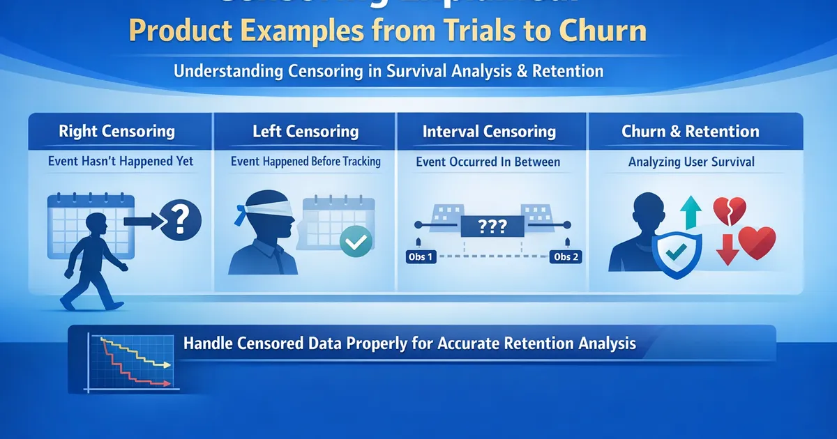
A practical guide to understanding censoring in survival analysis. Learn the different types of censoring, why it matters for retention analysis, and how to identify and handle censoring in your product data.
Quick Hits
- •Censoring = incomplete information about when the event occurred
- •Right censoring: Event hasn't happened YET (most common in tech)
- •Left censoring: Event happened BEFORE we started watching
- •Interval censoring: Event happened BETWEEN two observation points
- •Ignoring censoring biases your estimates - survival methods handle it properly
TL;DR
Censoring happens when you don't observe the exact event time—you only know it happened before, after, or within a window. In retention analysis, most censoring is "right censoring": the user hasn't churned yet, so you know they've survived at least until now. This isn't missing data to throw away—it's partial information that survival methods use correctly. Ignoring censoring leads to biased results.
What Is Censoring?
The Core Idea
Censoring occurs when you have incomplete information about when an event occurred.
You know something about the timing, but not the exact event time.
Types of Censoring
| Type | What You Know | Product Example |
|---|---|---|
| Right | Event hasn't happened yet | User is still active at day 60 |
| Left | Event happened before observation | User already churned when tracking started |
| Interval | Event happened between two times | User was active Monday, gone Friday |
Right Censoring (Most Common)
Definition
You observe the user until a certain time, and they haven't experienced the event yet.
Where = true event time, = censoring time.
What you know: The event time is greater than the observation time.
Causes in Product Analytics
-
Administrative censoring: Your analysis has a cutoff date; active users are censored at that date.
-
Staggered entry: Users signed up at different times; recent signups have less observation time.
-
Loss to follow-up: User deleted their account, switched devices, or otherwise disappeared for non-event reasons.
Example
| User | Signup | Last Seen | Status | Interpretation |
|---|---|---|---|---|
| A | Day 0 | Day 30 (churned) | Event | Churned at day 30 |
| B | Day 0 | Day 60 (active) | Censored | Survived at least 60 days |
| C | Day 30 | Day 90 (active) | Censored | Survived at least 60 days |
| D | Day 0 | Day 45 (deleted) | Censored | Survived at least 45 days |
Left Censoring
Definition
The event occurred before observation began—you missed it.
Where = true event time, = left censoring time (start of observation).
Causes in Product Analytics
-
Pre-existing conditions: User already churned from a previous product version before your new tracking started.
-
Retroactive analysis: You're analyzing historical data, but event tracking started late.
-
Delayed measurement: "Time since last purchase" for users whose first observed purchase wasn't their first-ever.
Example
You want to analyze "time from signup to first purchase," but purchase tracking only started 6 months ago.
| User | Signup | First Purchase | Status |
|---|---|---|---|
| A | 12 months ago | 10 months ago | Left censored (T < 6 months ago) |
| B | 3 months ago | 1 month ago | Observed (T = 2 months) |
| C | 5 months ago | Not yet | Right censored |
User A's first purchase was before tracking—you know it happened, but not exactly when.
Interval Censoring
Definition
You know the event happened between two observation times, but not exactly when.
Where = last known "no event," = first known "event occurred."
Causes in Product Analytics
-
Periodic observation: You check status weekly/monthly, so you only know events happened between checks.
-
Batch processing: Data updates daily; intraday timing is lost.
-
Survey-based measurement: "Have you used the product in the last 30 days?"
Example
Weekly activity checks:
| User | Week 1 | Week 2 | Week 3 | Status |
|---|---|---|---|---|
| A | Active | Active | Inactive | Interval (2, 3] |
| B | Active | Active | Active | Right censored at 3 |
| C | Active | Inactive | — | Interval (1, 2] |
You know User A churned sometime between week 2 and week 3, but not exactly when.
Why Censoring Matters
The Naive (Wrong) Approach
What analysts often do: Only analyze users who experienced the event.
"Average time to churn among churned users is 45 days."
What's wrong:
- Ignores users who survived longer than 45 days and haven't churned yet
- Biases estimate downward
- Gets worse with more censoring
The Correct Approach
Use survival methods (Kaplan-Meier, Cox) that properly account for censored observations.
Censored users contribute information: "They survived at least until censoring time."
Informative vs. Non-Informative Censoring
Non-Informative Censoring (Assumption)
Censoring is unrelated to the event risk.
Examples:
- Administrative end of study (all users censored same day)
- Random loss to follow-up (unrelated to churn probability)
Why it matters: Survival methods assume non-informative censoring. If this holds, estimates are unbiased.
Informative Censoring (Problem)
Censoring is related to event risk.
Examples:
- Users who are about to churn delete their accounts first
- Users who dislike the product also have missing data
- Power users who stick around are also more likely to respond to surveys
Why it matters: If high-risk users are systematically censored, your survival estimates are biased upward (you think retention is better than it is).
Identifying Censoring in Your Data
Step 1: Define the Event
Clearly define what constitutes the event:
- Churn: No activity in 30 days? Account deletion? Subscription cancellation?
- Conversion: First purchase? Subscription start?
Step 2: Identify Observation Windows
For each user:
- When did observation start? (signup, feature launch, etc.)
- When did observation end? (event time or censoring time)
- What was the status? (event or censored)
Step 3: Create Event Indicator
# Example: Churn defined as no activity for 30+ days
data['churn_date'] = data.apply(lambda r:
    r['last_activity'] if (today - r['last_activity']).days > 30 else pd.NaT,
    axis=1
)

# Observation time
data['observation_time'] = np.where(
    data['churn_date'].notna(),
    (data['churn_date'] - data['signup_date']).dt.days,  # Event time
    (today - data['signup_date']).dt.days  # Censoring time
)

# Event indicator
data['event'] = data['churn_date'].notna().astype(int)
Code: Handling Censoring
Python
import numpy as np
import pandas as pd
from lifelines import KaplanMeierFitter
import matplotlib.pyplot as plt


def prepare_survival_data(data, signup_col, event_col, event_date_col,
                          analysis_date=None):
    """
    Prepare data for survival analysis with proper censoring.

    Parameters:
    -----------
    data : pd.DataFrame
        Raw data
    signup_col : str
        Column with signup/start date
    event_col : str
        Column with event indicator (1=event, 0=active)
    event_date_col : str
        Column with event date (NaT if censored)
    analysis_date : datetime, optional
        Cutoff date for analysis (default: today)

    Returns:
    --------
    DataFrame with time and event columns ready for survival analysis
    """
    if analysis_date is None:
        analysis_date = pd.Timestamp.today()

    df = data.copy()

    # Calculate observation time
    df['_time'] = np.where(
        df[event_col] == 1,
        (df[event_date_col] - df[signup_col]).dt.days,
        (analysis_date - df[signup_col]).dt.days
    )

    # Handle negative times (should not exist)
    df['_time'] = df['_time'].clip(lower=0)

    # Event indicator
    df['_event'] = df[event_col]

    # Summary
    n_total = len(df)
    n_events = df['_event'].sum()
    n_censored = n_total - n_events

    print(f"Survival Data Summary")
    print(f"  Total observations: {n_total}")
    print(f"  Events: {n_events} ({n_events/n_total:.1%})")
    print(f"  Censored: {n_censored} ({n_censored/n_total:.1%})")
    print(f"  Observation time range: {df['_time'].min():.0f} - {df['_time'].max():.0f} days")

    return df[['_time', '_event']]


def visualize_censoring(data, n_sample=50, figsize=(12, 8)):
    """
    Create a swimmer plot showing censoring patterns.
    """
    # Sample data for visualization
    sample = data.sample(min(n_sample, len(data)), random_state=42).sort_values('_time')
    sample = sample.reset_index(drop=True)

    fig, ax = plt.subplots(figsize=figsize)

    for i, row in sample.iterrows():
        color = 'red' if row['_event'] == 1 else 'blue'
        marker = 'o' if row['_event'] == 1 else '|'

        # Draw line from 0 to observation time
        ax.hlines(i, 0, row['_time'], colors='gray', linewidth=1)
        # Draw endpoint
        ax.scatter(row['_time'], i, color=color, marker=marker, s=50)

    ax.set_xlabel('Days')
    ax.set_ylabel('User')
    ax.set_title('Censoring Pattern\n(Red dots = Events, Blue lines = Censored)')

    # Legend
    ax.scatter([], [], color='red', marker='o', label='Event')
    ax.scatter([], [], color='blue', marker='|', label='Censored')
    ax.legend(loc='lower right')

    return fig


def demonstrate_censoring_bias(data, time_col='_time', event_col='_event'):
    """
    Show how ignoring censoring biases estimates.
    """
    # Naive: only use events
    events_only = data[data[event_col] == 1]
    naive_mean = events_only[time_col].mean()
    naive_median = events_only[time_col].median()

    # Correct: Kaplan-Meier
    kmf = KaplanMeierFitter()
    kmf.fit(data[time_col], data[event_col])
    km_median = kmf.median_survival_time_

    print("Comparison: Naive vs Survival Analysis")
    print("=" * 50)
    print(f"\nNaive (events only):")
    print(f"  Mean time to event: {naive_mean:.1f} days")
    print(f"  Median time to event: {naive_median:.1f} days")
    print(f"  Sample size: {len(events_only)}")

    print(f"\nKaplan-Meier (correct):")
    print(f"  Median survival time: {km_median:.1f} days")
    print(f"  Sample size: {len(data)}")

    print(f"\nBias in naive estimate: {naive_median - km_median:.1f} days")
    print("(Negative = naive underestimates survival)")

    return {
        'naive_median': naive_median,
        'km_median': km_median,
        'bias': naive_median - km_median
    }


# Example
if __name__ == "__main__":
    np.random.seed(42)
    n = 500

    # Simulate data with censoring
    signup_dates = pd.Timestamp('2024-01-01') + pd.to_timedelta(
        np.random.uniform(0, 180, n), unit='D'
    )

    # True survival times (exponential with median ~60 days)
    true_survival = np.random.exponential(60, n)

    # Analysis date
    analysis_date = pd.Timestamp('2024-07-01')

    # Event dates (churn)
    event_dates = signup_dates + pd.to_timedelta(true_survival, unit='D')

    # Censoring: event after analysis date
    event_indicator = (event_dates <= analysis_date).astype(int)
    event_dates = event_dates.where(event_indicator == 1)

    # Create DataFrame
    raw_data = pd.DataFrame({
        'signup_date': signup_dates,
        'churned': event_indicator,
        'churn_date': event_dates
    })

    # Prepare for survival analysis
    surv_data = prepare_survival_data(
        raw_data, 'signup_date', 'churned', 'churn_date',
        analysis_date=analysis_date
    )

    # Visualize censoring
    fig = visualize_censoring(surv_data)
    plt.tight_layout()

    # Demonstrate bias
    print("\n")
    demonstrate_censoring_bias(surv_data)

    plt.show()
R
library(tidyverse)
library(survival)
library(survminer)


prepare_survival_data <- function(data, signup_col, event_col, event_date_col,
                                   analysis_date = Sys.Date()) {
    #' Prepare data for survival analysis with proper censoring

    data %>%
        mutate(
            time = ifelse(
                .data[[event_col]] == 1,
                as.numeric(difftime(.data[[event_date_col]], .data[[signup_col]], units = "days")),
                as.numeric(difftime(analysis_date, .data[[signup_col]], units = "days"))
            ),
            time = pmax(time, 0),
            event = .data[[event_col]]
        )
}


demonstrate_censoring_bias <- function(data, time_col = "time", event_col = "event") {
    #' Show how ignoring censoring biases estimates

    # Naive: events only
    events_only <- data %>% filter(.data[[event_col]] == 1)
    naive_median <- median(events_only[[time_col]])

    # Correct: Kaplan-Meier
    surv_obj <- Surv(data[[time_col]], data[[event_col]])
    km_fit <- survfit(surv_obj ~ 1)
    km_median <- summary(km_fit)$table["median"]

    cat("Comparison: Naive vs Survival Analysis\n")
    cat(strrep("=", 50), "\n")
    cat(sprintf("\nNaive (events only): %.1f days (n=%d)\n", naive_median, nrow(events_only)))
    cat(sprintf("Kaplan-Meier: %.1f days (n=%d)\n", km_median, nrow(data)))
    cat(sprintf("Bias: %.1f days\n", naive_median - km_median))

    list(naive_median = naive_median, km_median = km_median)
}
Common Mistakes
Mistake 1: Excluding Censored Observations
Wrong: "I only analyzed users who churned to get the average time to churn."
Right: Use all users. Censored users provide information about minimum survival.
Mistake 2: Treating Censoring Time as Event Time
Wrong: Coding censored users' observation time as their churn time.
Right: Track both time and event indicator separately.
Mistake 3: Ignoring Informative Censoring
Wrong: Assuming all censoring is random when it's not.
Right: Think about why users are censored. If it's related to the outcome, consider sensitivity analyses.
Related Methods
- Time-to-Event and Retention Analysis (Pillar) - Full survival framework
- Kaplan-Meier Curves - Handling censoring visually
- Cox Proportional Hazards - Regression with censoring
- Missing Data Guide - Related concepts
Key Takeaway
Censoring is incomplete information about event times, not missing data to exclude. Right censoring (event hasn't happened yet) is most common in product analytics—it tells you the user survived at least until the censoring time. Survival methods (Kaplan-Meier, Cox) properly incorporate this partial information. Ignoring censoring by analyzing only events biases your estimates downward. Always prepare your data with both observation time and event indicator, and use appropriate survival analysis methods.
References
- https://www.ncbi.nlm.nih.gov/pmc/articles/PMC3275994/
- https://lifelines.readthedocs.io/en/latest/Survival%20Analysis%20intro.html
- https://www.bmj.com/content/317/7156/468
- Leung, K. M., Elashoff, R. M., & Afifi, A. A. (1997). Censoring issues in survival analysis. *Annual Review of Public Health*, 18, 83-104.
- lifelines documentation. Survival Analysis Introduction.
- Altman, D. G., & Bland, J. M. (1998). Time to event (survival) data. *BMJ*, 317(7156), 468-469.
Frequently Asked Questions
Why can't I just exclude censored observations?
What's the most common type of censoring in product analytics?
Does censoring always come from the right?
Key Takeaway
Censoring occurs when you have incomplete information about event times. It's not missing data—it's partial information that survival methods use correctly. Right-censored observations tell you 'the user survived at least this long,' which is valuable for estimation. Always use survival methods with censored data; ignoring censoring biases results.