Contents
Regression vs. t-Test vs. ANOVA: The Unifying View (and When the Simpler Tool Suffices)
Understand how t-tests, ANOVA, and regression are all the same underlying model. Learn when to use the simpler approach and when regression's flexibility is worth it.
Quick Hits
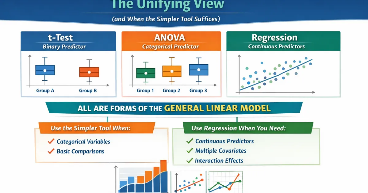
- •T-tests, ANOVA, and regression are all special cases of the general linear model
- •A two-sample t-test is regression with one binary predictor
- •One-way ANOVA is regression with one categorical predictor (dummy coded)
- •Use the simpler tool when it suffices - it's more interpretable
- •Use regression when you need: continuous predictors, multiple covariates, or interactions
TL;DR
T-tests, ANOVA, and linear regression are all special cases of the general linear model. A two-sample t-test is regression with one binary predictor. One-way ANOVA is regression with one categorical predictor. Understanding this unification helps you see that the "choice" between them is about presentation, not statistics. Use the simpler tool when it fits your problem; switch to regression when you need continuous predictors, covariates, or complex comparisons.
The Big Picture
All these tests fit the same underlying model:
Where:
- Y is your outcome
- X is your design matrix (encodes groups/predictors)
- is your coefficients (means or effects)
- ε is error (assumed normal, constant variance)
The "choice" between tests is really about:
- How you construct X (dummy coding, effect coding, etc.)
- How you report results (means vs. coefficients, F vs. t)
- How interpretable the output is for your audience
One-Sample t-Test = Regression with Intercept Only
The t-Test
Test whether mean differs from a value (usually 0):
The Regression
is the mean of . Testing is identical to the one-sample t-test.
Demonstration
import numpy as np
from scipy import stats
import statsmodels.formula.api as smf
import pandas as pd

np.random.seed(42)
y = np.random.normal(5, 2, 100)

# One-sample t-test
t_stat, p_value = stats.ttest_1samp(y, 0)
print(f"T-test: t = {t_stat:.4f}, p = {p_value:.4f}")

# Regression (intercept only)
data = pd.DataFrame({'y': y})
model = smf.ols('y ~ 1', data=data).fit()
print(f"Regression: t = {model.tvalues['Intercept']:.4f}, p = {model.pvalues['Intercept']:.4f}")
print(f"Coefficient (mean) = {model.params['Intercept']:.4f}, Sample mean = {y.mean():.4f}")
Output:
T-test: t = 24.8503, p = 0.0000
Regression: t = 24.8503, p = 0.0000
Coefficient (mean) = 4.9397, Sample mean = 4.9397
Two-Sample t-Test = Regression with Binary Predictor
The t-Test
Compare means of two groups:
The Regression
Where Group = 0 for control, 1 for treatment.
Interpretation:
- = mean of control group (when Group = 0)
- = difference in means (treatment - control)
- Testing is identical to the two-sample t-test
Demonstration
# Generate data
np.random.seed(42)
control = np.random.normal(10, 3, 50)
treatment = np.random.normal(12, 3, 50)

# Two-sample t-test (equal variance)
t_stat, p_value = stats.ttest_ind(control, treatment)
print(f"T-test: t = {t_stat:.4f}, p = {p_value:.4f}")

# Regression
data = pd.DataFrame({
    'y': np.concatenate([control, treatment]),
    'group': [0]*50 + [1]*50
})
model = smf.ols('y ~ group', data=data).fit()
print(f"Regression: t = {model.tvalues['group']:.4f}, p = {model.pvalues['group']:.4f}")
print(f"\nControl mean: {control.mean():.4f}")
print(f"Intercept (β₀): {model.params['Intercept']:.4f}")
print(f"Difference: {treatment.mean() - control.mean():.4f}")
print(f"Group coefficient (β₁): {model.params['group']:.4f}")
Note: The equal-variance t-test matches regression. Welch's t-test (unequal variance) requires heteroscedasticity-robust standard errors in regression.
One-Way ANOVA = Regression with Categorical Predictor
ANOVA
Compare means across k groups:
Regression with Dummy Variables
For k groups, create k-1 dummy variables:
Interpretation:
- = mean of reference group
- = difference between group j and reference group
The F-Test Connection
ANOVA reports an F-statistic testing all groups equal. In regression:
- The overall F-test for the model tests the same hypothesis
- Individual t-tests for dummy coefficients test pairwise differences from reference
Demonstration
# Three groups
np.random.seed(42)
group_a = np.random.normal(10, 2, 40)
group_b = np.random.normal(12, 2, 40)
group_c = np.random.normal(11, 2, 40)

# One-way ANOVA
f_stat, p_value = stats.f_oneway(group_a, group_b, group_c)
print(f"ANOVA: F = {f_stat:.4f}, p = {p_value:.4f}")

# Regression with dummies
data = pd.DataFrame({
    'y': np.concatenate([group_a, group_b, group_c]),
    'group': ['A']*40 + ['B']*40 + ['C']*40
})
model = smf.ols('y ~ C(group)', data=data).fit()
print(f"Regression F-test: F = {model.fvalue:.4f}, p = {model.f_pvalue:.4f}")

print("\nGroup means:")
print(f"  A: {group_a.mean():.4f}")
print(f"  B: {group_b.mean():.4f}")
print(f"  C: {group_c.mean():.4f}")

print("\nRegression coefficients:")
print(f"  Intercept (Group A mean): {model.params['Intercept']:.4f}")
print(f"  B vs A: {model.params['C(group)[T.B]']:.4f}")
print(f"  C vs A: {model.params['C(group)[T.C]']:.4f}")
Two-Way ANOVA = Regression with Two Categorical Predictors
Two-Way ANOVA
Tests:
- Main effect of Factor A
- Main effect of Factor B
- A × B Interaction
Regression Equivalent
With appropriate dummy coding for categorical variables.
# Regression for two-way ANOVA
model = smf.ols('y ~ C(factor_a) * C(factor_b)', data=data).fit()

# ANOVA table from regression
import statsmodels.api as sm
anova_table = sm.stats.anova_lm(model, typ=2)  # Type II SS
print(anova_table)
Paired t-Test = Regression on Differences
Paired t-Test
Compare paired observations (before/after, matched pairs):
Regression Equivalent
Create difference variable, then one-sample test:
Testing is the paired t-test.
Alternative: Repeated Measures Regression
# Mixed effects model approach
import statsmodels.formula.api as smf

# Long format data with subject ID
model = smf.mixedlm('y ~ time', data=data, groups=data['subject_id']).fit()
The Equivalence Table
| Simple Test | Regression Equivalent |
|---|---|
| One-sample t-test | Y ~ 1 (intercept only) |
| Two-sample t-test | Y ~ group (binary) |
| Paired t-test | Y_diff ~ 1 or mixed model |
| One-way ANOVA | Y ~ factor (dummy coded) |
| Two-way ANOVA | Y ~ A * B |
| ANCOVA | Y ~ factor + covariate |
| Correlation test | Y ~ X (standardized) |
| Simple regression | Y ~ X |
| Multiple regression | Y ~ X1 + X2 + ... |
Code: Demonstrating Equivalence
Python
import numpy as np
import pandas as pd
from scipy import stats
import statsmodels.formula.api as smf
import statsmodels.api as sm


np.random.seed(42)

# --- Two-sample t-test vs regression ---
control = np.random.normal(100, 15, 50)
treatment = np.random.normal(110, 15, 50)

# T-test
t_result = stats.ttest_ind(control, treatment)

# Equivalent regression
data = pd.DataFrame({
    'y': np.concatenate([control, treatment]),
    'group': [0]*50 + [1]*50
})
model = smf.ols('y ~ group', data=data).fit()
The t-test and regression produce the same t-statistic and p-value. The regression coefficient equals the mean difference between groups.
# --- One-way ANOVA vs regression ---
group_a = np.random.normal(100, 15, 40)
group_b = np.random.normal(110, 15, 40)
group_c = np.random.normal(105, 15, 40)

# ANOVA
f_result = stats.f_oneway(group_a, group_b, group_c)

# Equivalent regression
data = pd.DataFrame({
    'y': np.concatenate([group_a, group_b, group_c]),
    'group': ['A']*40 + ['B']*40 + ['C']*40
})
model = smf.ols('y ~ C(group)', data=data).fit()
The F-statistic and p-value are identical from both approaches. ANOVA is just regression with categorical predictors.
# --- Paired t-test vs regression on differences ---
before = np.random.normal(100, 15, 30)
after = before + np.random.normal(5, 10, 30)

# Paired t-test
t_result = stats.ttest_rel(before, after)

# Equivalent regression on differences
diff = after - before
data = pd.DataFrame({'diff': diff})
model = smf.ols('diff ~ 1', data=data).fit()
A paired t-test is equivalent to testing whether the intercept of a regression on differences is zero. Same t-statistic, same p-value.
R
library(tidyverse)


demonstrate_equivalence <- function() {
    set.seed(42)

    # Two-sample case
    cat(strrep("=", 60), "\n")
    cat("TWO-SAMPLE T-TEST vs REGRESSION\n")
    cat(strrep("=", 60), "\n")

    control <- rnorm(50, 100, 15)
    treatment <- rnorm(50, 110, 15)

    # T-test
    t_result <- t.test(control, treatment, var.equal = TRUE)
    cat(sprintf("\nTwo-sample t-test:\n"))
    cat(sprintf("  t = %.4f\n", t_result$statistic))
    cat(sprintf("  p = %.4f\n", t_result$p.value))

    # Regression
    data <- tibble(
        y = c(control, treatment),
        group = factor(c(rep(0, 50), rep(1, 50)))
    )
    model <- lm(y ~ group, data = data)
    cat(sprintf("\nRegression:\n"))
    cat(sprintf("  t = %.4f\n", summary(model)$coefficients["group1", "t value"]))
    cat(sprintf("  p = %.4f\n", summary(model)$coefficients["group1", "Pr(>|t|)"]))

    # One-way ANOVA case
    cat("\n", strrep("=", 60), "\n")
    cat("ONE-WAY ANOVA vs REGRESSION\n")
    cat(strrep("=", 60), "\n")

    group_a <- rnorm(40, 100, 15)
    group_b <- rnorm(40, 110, 15)
    group_c <- rnorm(40, 105, 15)

    data <- tibble(
        y = c(group_a, group_b, group_c),
        group = factor(c(rep("A", 40), rep("B", 40), rep("C", 40)))
    )

    # ANOVA
    aov_result <- aov(y ~ group, data = data)
    cat(sprintf("\nOne-way ANOVA:\n"))
    cat(sprintf("  F = %.4f\n", summary(aov_result)[[1]]["group", "F value"]))
    cat(sprintf("  p = %.4f\n", summary(aov_result)[[1]]["group", "Pr(>F)"]))

    # Regression
    model <- lm(y ~ group, data = data)
    cat(sprintf("\nRegression:\n"))
    cat(sprintf("  F = %.4f\n", summary(model)$fstatistic[1]))
    cat(sprintf("  p = %.4f\n", pf(summary(model)$fstatistic[1],
                                   summary(model)$fstatistic[2],
                                   summary(model)$fstatistic[3],
                                   lower.tail = FALSE)))
}


demonstrate_equivalence()
When to Use Which
Use t-Test When
- You have two groups
- No covariates to control for
- You want simple, recognizable output
- Your audience thinks in terms of "comparing two means"
Use ANOVA When
- You have multiple (3+) categorical groups
- No continuous predictors
- You want to decompose variance (between vs. within)
- Your audience is familiar with ANOVA tables
Use Regression When
- You have continuous predictors
- You need to control for covariates
- You want custom contrasts (not just vs. reference)
- You have complex interactions
- You need to include both categorical and continuous predictors
- You want coefficient-based interpretation
Advantages of the Regression Framing
1. Flexibility
Regression handles any combination of:
- Continuous predictors
- Categorical predictors (with dummy coding)
- Interactions
- Covariates
2. Custom Contrasts
With regression, you can easily test specific comparisons:
# Test: Is the average of B and C different from A?
model = smf.ols('y ~ C(group, Treatment("A"))', data=data).fit()

# Custom contrast matrix
from patsy.contrasts import ContrastMatrix
# ... define specific contrasts
3. Extends to GLMs
The same framework extends to:
- Logistic regression (binary outcomes)
- Poisson regression (count outcomes)
- Any generalized linear model
4. Clearer About What You're Testing
Regression output shows exactly what comparison each coefficient represents, rather than hiding it in sum-of-squares decomposition.
Common Misconceptions
"Regression requires normality of X"
False. Regression assumes normality of residuals (errors), not predictors. You can use regression with any distribution of X.
"ANOVA is for experiments, regression is for observational data"
False. Both can be used for either. The model is the same; the interpretation differs based on study design.
"I need to check normality of my groups for ANOVA"
Partially false. You need approximate normality of residuals (within each group). With large samples, this matters less due to CLT.
"T-tests are less powerful than regression"
False. They're identical (same test). Regression might have more power if you include relevant covariates that reduce error variance.
Related Methods
- Regression for Analysts (Pillar) - Complete regression framework
- One-Way ANOVA - ANOVA details
- Welch's t-Test vs. Student's t-Test - Which t-test to use
- Interaction Terms - Factorial designs in regression
Key Takeaway
T-tests, ANOVA, and regression are all the general linear model with different interfaces. Understanding this unification demystifies statistical testing: there's one underlying framework, and the "different tests" are just different ways of specifying and presenting it. Use the simplest tool that fits your problem (t-test for two groups, ANOVA for multiple groups with categorical predictors), but know that regression is there when you need its flexibility (continuous predictors, covariates, custom contrasts). The p-values and statistical conclusions will be identical.
References
- https://lindeloev.github.io/tests-as-linear/
- https://www.amazon.com/Statistical-Rethinking-Bayesian-Examples-Chapman/dp/036713991X
- https://www.sciencedirect.com/science/article/pii/S0022103117307746
- Lindeløv, J. K. (2019). Common statistical tests are linear models. Online tutorial.
- McElreath, R. (2020). Statistical rethinking: A Bayesian course with examples in R and Stan (2nd ed.). CRC Press.
- Judd, C. M., McClelland, G. H., & Ryan, C. S. (2017). Data analysis: A model comparison approach (3rd ed.). Routledge.
Frequently Asked Questions
Will I get different results from a t-test vs. regression?
Why would I use ANOVA if it's just regression?
When should I switch from ANOVA to regression?
Key Takeaway
T-tests, ANOVA, and regression are all the general linear model with different packaging. Understanding this unification helps you see when the simpler tool suffices (categorical predictors, no covariates) and when regression's flexibility is needed (continuous predictors, multiple controls, custom contrasts).