Contents
One-Way ANOVA: Assumptions, Effect Sizes, and Proper Reporting
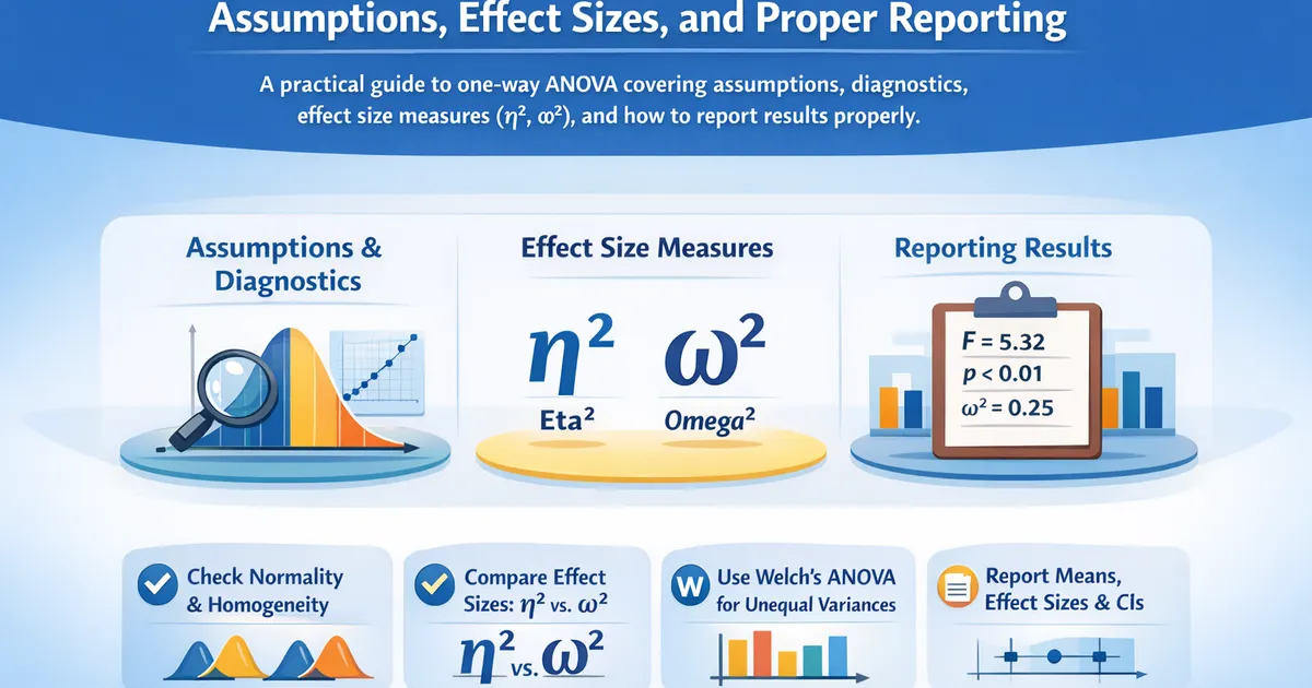
A practical guide to one-way ANOVA covering assumptions, diagnostics, effect size measures (eta-squared, omega-squared), and how to report results properly.
Quick Hits
- •ANOVA is robust to moderate normality violations with equal sample sizes
- •Unequal variances are more problematic than non-normality—use Welch's ANOVA
- •Eta-squared overestimates population effect size; omega-squared is less biased
- •Always report effect sizes and confidence intervals, not just F and p
TL;DR
One-way ANOVA compares means across groups by partitioning variance. It's robust to moderate normality violations but sensitive to unequal variances—use Welch's ANOVA when variances differ. Always report effect sizes (omega-squared preferred over eta-squared) alongside F-statistics. A complete report includes group means, F-statistic, degrees of freedom, p-value, effect size with interpretation, and post-hoc results.
The ANOVA Framework
ANOVA partitions total variance into between-group and within-group components:
The F-statistic compares these:
Where k = number of groups, N = total sample size.
Large F means between-group variance exceeds within-group variance more than expected by chance.
Assumptions
1. Independence
Observations must be independent—one person's score doesn't affect another's.
Violations: Repeated measures on same subjects, clustered data (students in classrooms), time series.
Consequence: Standard errors are wrong; p-values are unreliable.
Solution: Use repeated-measures ANOVA, mixed models, or cluster-robust standard errors.
2. Normality
Data within each group should be approximately normally distributed.
How to check:
import numpy as np
import matplotlib.pyplot as plt
from scipy import stats

def check_normality(groups, group_names=None):
    """Visual and statistical normality checks."""
    k = len(groups)
    if group_names is None:
        group_names = [f'Group {i+1}' for i in range(k)]

    fig, axes = plt.subplots(2, k, figsize=(4*k, 8))

    for i, (g, name) in enumerate(zip(groups, group_names)):
        # Histogram
        axes[0, i].hist(g, bins='auto', edgecolor='black', alpha=0.7)
        axes[0, i].set_title(f'{name} Histogram')

        # Q-Q plot
        stats.probplot(g, dist="norm", plot=axes[1, i])
        axes[1, i].set_title(f'{name} Q-Q Plot')

    plt.tight_layout()
    return fig
Robustness: ANOVA is robust to non-normality with:
- Equal or near-equal sample sizes
- n > 15-20 per group
- Moderate skewness (|skew| < 2)
When it matters: Small samples, severe skewness, unequal group sizes.
3. Homogeneity of Variance (Homoscedasticity)
Groups should have similar variances.
How to check:
from scipy.stats import levene, bartlett

def check_variance_homogeneity(groups):
    """Test for equal variances."""
    # Levene's test (robust to non-normality)
    levene_stat, levene_p = levene(*groups, center='median')

    # Variance ratio (largest/smallest)
    variances = [np.var(g, ddof=1) for g in groups]
    variance_ratio = max(variances) / min(variances)

    return {
        'levene_statistic': levene_stat,
        'levene_p': levene_p,
        'variance_ratio': variance_ratio,
        'rule_of_thumb': 'OK' if variance_ratio < 3 else 'Concern'
    }
Rule of thumb: Variance ratio < 3 is usually acceptable. Larger ratios warrant Welch's ANOVA.
Consequence of violation: Type I error inflation when smaller groups have larger variance; conservatism when larger groups have larger variance.
Effect Sizes
P-values tell you whether an effect exists; effect sizes tell you how large it is.
Eta-Squared (η²)
Proportion of variance explained by group membership:
def eta_squared(groups):
    """Calculate eta-squared."""
    grand_mean = np.mean(np.concatenate(groups))

    ss_between = sum(len(g) * (np.mean(g) - grand_mean)**2 for g in groups)
    ss_total = sum(np.sum((g - grand_mean)**2) for g in groups)

    return ss_between / ss_total
Problem: Eta-squared is positively biased—it overestimates the population effect size, especially with small samples.
Omega-Squared (ω²)
Less biased estimate of population effect size:
def omega_squared(groups):
    """Calculate omega-squared (less biased than eta-squared)."""
    k = len(groups)
    n_total = sum(len(g) for g in groups)
    grand_mean = np.mean(np.concatenate(groups))

    ss_between = sum(len(g) * (np.mean(g) - grand_mean)**2 for g in groups)
    ss_within = sum(np.sum((g - np.mean(g))**2) for g in groups)
    ss_total = ss_between + ss_within

    ms_within = ss_within / (n_total - k)

    omega_sq = (ss_between - (k - 1) * ms_within) / (ss_total + ms_within)

    return max(0, omega_sq)  # Can't be negative
Interpreting Effect Sizes
| Effect Size | η² / ω² | Interpretation |
|---|---|---|
| Small | 0.01 | 1% of variance explained |
| Medium | 0.06 | 6% of variance explained |
| Large | 0.14 | 14% of variance explained |
Context matters: A "small" effect in psychology might be huge in medicine. Interpret relative to your field and practical significance.
Partial Eta-Squared
In factorial designs, partial η² isolates the effect of one factor:
This is what most software reports by default.
Complete ANOVA Analysis
import numpy as np
from scipy import stats
import pandas as pd

def complete_anova(groups, group_names=None, alpha=0.05):
    """
    Complete one-way ANOVA analysis with all components.
    """
    if group_names is None:
        group_names = [f'Group {i+1}' for i in range(len(groups))]

    k = len(groups)
    n_total = sum(len(g) for g in groups)
    grand_mean = np.mean(np.concatenate(groups))

    # Sums of squares
    ss_between = sum(len(g) * (np.mean(g) - grand_mean)**2 for g in groups)
    ss_within = sum(np.sum((g - np.mean(g))**2) for g in groups)
    ss_total = ss_between + ss_within

    # Degrees of freedom
    df_between = k - 1
    df_within = n_total - k
    df_total = n_total - 1

    # Mean squares
    ms_between = ss_between / df_between
    ms_within = ss_within / df_within

    # F-statistic and p-value
    f_stat = ms_between / ms_within
    p_value = 1 - stats.f.cdf(f_stat, df_between, df_within)

    # Effect sizes
    eta_sq = ss_between / ss_total
    omega_sq = max(0, (ss_between - df_between * ms_within) / (ss_total + ms_within))

    # Confidence interval for omega-squared (approximate)
    # Using non-central F distribution

    # Group statistics
    group_stats = pd.DataFrame({
        'Group': group_names,
        'n': [len(g) for g in groups],
        'Mean': [np.mean(g) for g in groups],
        'SD': [np.std(g, ddof=1) for g in groups],
        'SE': [np.std(g, ddof=1) / np.sqrt(len(g)) for g in groups]
    })

    # ANOVA table
    anova_table = pd.DataFrame({
        'Source': ['Between Groups', 'Within Groups', 'Total'],
        'SS': [ss_between, ss_within, ss_total],
        'df': [df_between, df_within, df_total],
        'MS': [ms_between, ms_within, np.nan],
        'F': [f_stat, np.nan, np.nan],
        'p': [p_value, np.nan, np.nan]
    })

    return {
        'group_stats': group_stats,
        'anova_table': anova_table,
        'f_statistic': f_stat,
        'p_value': p_value,
        'df_between': df_between,
        'df_within': df_within,
        'eta_squared': eta_sq,
        'omega_squared': omega_sq,
        'significant': p_value < alpha
    }


# Example
np.random.seed(42)
control = np.random.normal(50, 10, 25)
treatment_a = np.random.normal(55, 10, 25)
treatment_b = np.random.normal(52, 10, 25)

result = complete_anova(
    [control, treatment_a, treatment_b],
    ['Control', 'Treatment A', 'Treatment B']
)

print("Group Statistics:")
print(result['group_stats'].to_string(index=False))
print("\nANOVA Table:")
print(result['anova_table'].to_string(index=False))
print(f"\nEffect Sizes:")
print(f"  η² = {result['eta_squared']:.3f}")
print(f"  ω² = {result['omega_squared']:.3f}")
Reporting Results
APA Style Format
A one-way ANOVA was conducted to compare the effect of treatment condition on test scores. There was a significant effect of treatment at the level for the three conditions, F(2, 72) = 4.52, , ω² = .086 [95% CI: .01, .19]. Post-hoc comparisons using Tukey's HSD indicated that Treatment A (M = 55.2, SD = 9.8) was significantly higher than Control (M = 50.1, SD = 10.2), . Treatment B (M = 52.3, SD = 10.1) did not differ significantly from either Control or Treatment A.
Elements to Include
- Test used: One-way ANOVA (or Welch's ANOVA)
- Purpose: What was compared
- F-statistic: F(df_between, df_within) = value
- P-value: Exact value or inequality
- Effect size: ω² or η² with interpretation
- Group means and SDs: For each group
- Post-hoc results: Which groups differ
Common Mistakes
- Reporting only F and p, no effect size
- Using η² but calling it ω²
- Not specifying which post-hoc test was used
- Reporting post-hoc without significant omnibus test
When to Use Welch's ANOVA
Use Welch's ANOVA when:
- Levene's test is significant ()
- Variance ratio exceeds 3
- You're uncertain about equal variances
- As a default (it's never worse than standard ANOVA)
from scipy.stats import alexandergovern

def welch_anova(groups):
    """Welch's ANOVA for unequal variances."""
    result = alexandergovern(*groups)
    return {
        'statistic': result.statistic,
        'p_value': result.pvalue
    }
Related Methods
- Comparing More Than Two Groups — The pillar guide
- Post-Hoc Tests: Tukey, Dunnett, Games-Howell — Following up significant ANOVA
- Visual Diagnostics for Group Comparisons — Checking assumptions visually
Key Takeaway
ANOVA is robust to moderate assumption violations, especially with balanced designs. Focus on effect sizes (omega-squared) and confidence intervals rather than just p-values. When variances differ, use Welch's ANOVA. A complete report includes group means and SDs, F-statistic with degrees of freedom, p-value, effect size with interpretation, and post-hoc results identifying which groups differ.
References
- https://www.jstor.org/stable/2529310
- https://psycnet.apa.org/record/2004-19012-003
- Glass, G. V., Peckham, P. D., & Sanders, J. R. (1972). Consequences of failure to meet assumptions underlying the fixed effects analyses of variance and covariance. *Review of Educational Research*, 42(3), 237-288.
- Olejnik, S., & Algina, J. (2003). Generalized eta and omega squared statistics: measures of effect size for some common research designs. *Psychological Methods*, 8(4), 434-447.
- Lakens, D. (2013). Calculating and reporting effect sizes to facilitate cumulative science. *Frontiers in Psychology*, 4, 863.
Frequently Asked Questions
How robust is ANOVA to normality violations?
What's the difference between eta-squared and omega-squared?
Should I test assumptions before running ANOVA?
Key Takeaway
ANOVA is robust to moderate assumption violations, especially with balanced designs. Focus on effect sizes (omega-squared) and confidence intervals rather than just p-values. When variances differ, use Welch's ANOVA. Report group means, effect sizes, and follow significant results with appropriate post-hoc tests.