Contents
Effect Sizes for Mean Differences: Cohen's d, Hedges' g, and Raw Differences
A practical guide to effect sizes for comparing means. Learn when to use standardized vs. raw effect sizes, how to calculate and interpret them, and how to report them properly.
Quick Hits
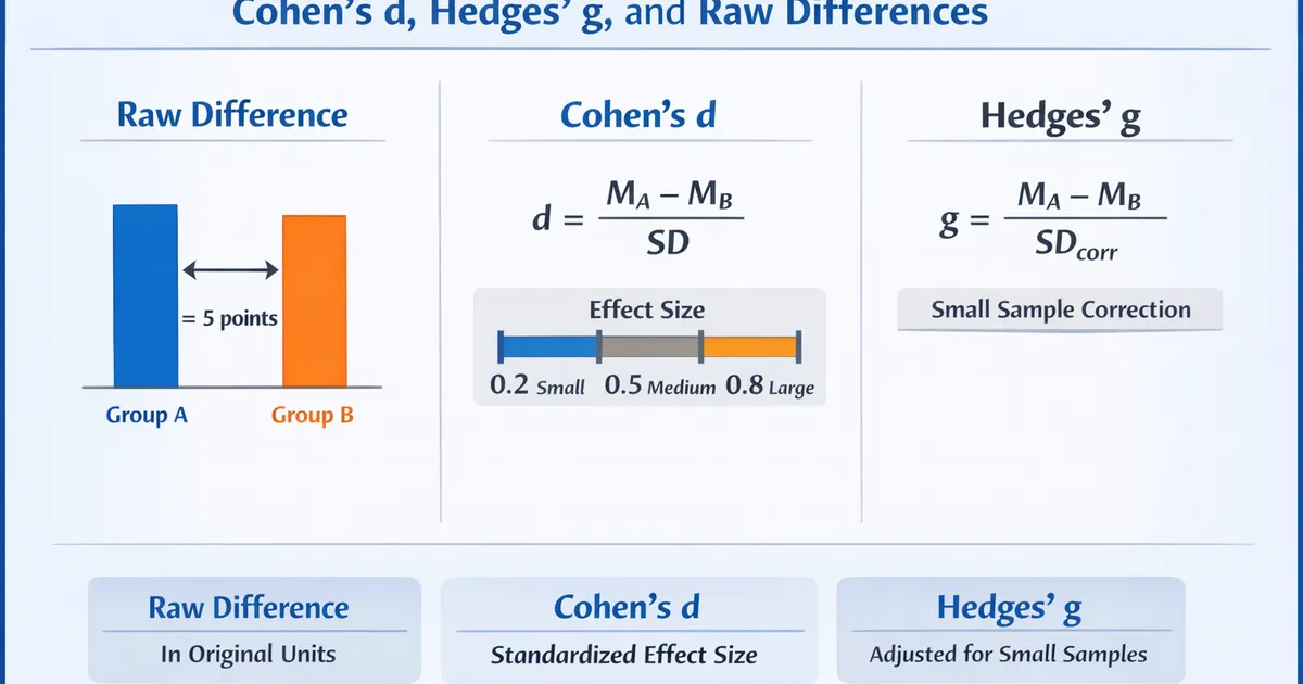
- •Raw differences are in original units; standardized (d, g) are in SD units
- •Cohen's d is biased upward for small samples; Hedges' g corrects this
- •Cohen's benchmarks (0.2, 0.5, 0.8) are guidelines, not rules
- •Always report raw differences for stakeholders; standardized for meta-analysis
TL;DR
Raw effect sizes tell you the actual difference in measurement units ("5 more clicks"). Standardized effect sizes (Cohen's d, Hedges' g) express differences in standard deviation units, enabling comparison across different scales. Use Hedges' g for small samples to correct Cohen's d's upward bias. Report raw differences for practical interpretation, standardized for meta-analyses and cross-study comparisons.
Raw (Unstandardized) Effect Sizes
The Basics
import numpy as np
from scipy import stats

def raw_effect_size(group1, group2, confidence=0.95):
    """
    Calculate raw effect size with confidence interval.
    """
    n1, n2 = len(group1), len(group2)
    m1, m2 = np.mean(group1), np.mean(group2)
    v1, v2 = np.var(group1, ddof=1), np.var(group2, ddof=1)

    # Difference
    diff = m2 - m1

    # Standard error (Welch's approach)
    se = np.sqrt(v1/n1 + v2/n2)

    # Degrees of freedom (Welch-Satterthwaite)
    num = (v1/n1 + v2/n2)**2
    denom = (v1/n1)**2/(n1-1) + (v2/n2)**2/(n2-1)
    df = num / denom

    # CI
    t_crit = stats.t.ppf(1 - (1-confidence)/2, df)
    ci = (diff - t_crit * se, diff + t_crit * se)

    # Percent change
    pct_change = diff / m1 * 100 if m1 != 0 else None

    return {
        'mean_1': m1,
        'mean_2': m2,
        'difference': diff,
        'se': se,
        'df': df,
        'ci': ci,
        'pct_change': pct_change
    }


# Example: Page load time (seconds)
np.random.seed(42)
old_system = np.random.normal(3.5, 0.8, 100)
new_system = np.random.normal(3.0, 0.7, 100)

result = raw_effect_size(old_system, new_system)

print("Raw Effect Size Example: Page Load Time")
print("-" * 50)
print(f"Old system: {result['mean_1']:.3f}s")
print(f"New system: {result['mean_2']:.3f}s")
print(f"Difference: {result['difference']:.3f}s")
print(f"95% CI: [{result['ci'][0]:.3f}s, {result['ci'][1]:.3f}s]")
print(f"Improvement: {result['pct_change']:.1f}%")
print()
print("This is immediately interpretable: ")
print(f"'The new system is {-result['difference']:.2f} seconds faster'")
When Raw is Best
Clear interpretable scale:
- Dollars saved/earned
- Time (seconds, days)
- Count of events
- Percentage points
Communicating to stakeholders:
- Business decisions need concrete numbers
- "d = 0.5" means nothing to executives
- "$12 more revenue per user" is actionable
Cost-benefit analysis:
- Need actual units to calculate ROI
- Implementation costs are in real units
- Standardized effects don't translate to dollars
Cohen's d: Standardized Effect Size
Calculation
where
def cohens_d(group1, group2, pooled=True):
    """
    Calculate Cohen's d.

    pooled=True: Use pooled SD (equal variance assumption)
    pooled=False: Use control group SD (Glass's delta)
    """
    n1, n2 = len(group1), len(group2)
    m1, m2 = np.mean(group1), np.mean(group2)
    v1, v2 = np.var(group1, ddof=1), np.var(group2, ddof=1)

    if pooled:
        # Pooled SD
        sp = np.sqrt(((n1-1)*v1 + (n2-1)*v2) / (n1 + n2 - 2))
        d = (m2 - m1) / sp
    else:
        # Glass's delta (control SD)
        d = (m2 - m1) / np.sqrt(v1)

    # Approximate CI for d
    se_d = np.sqrt((n1 + n2) / (n1 * n2) + d**2 / (2 * (n1 + n2)))
    ci = (d - 1.96 * se_d, d + 1.96 * se_d)

    return {
        'd': d,
        'se': se_d,
        'ci': ci
    }


# Example
np.random.seed(42)
control = np.random.normal(100, 15, 50)
treatment = np.random.normal(107.5, 15, 50)  # Half SD improvement

result = cohens_d(control, treatment)

print("Cohen's d Example")
print("-" * 40)
print(f"d = {result['d']:.3f}")
print(f"SE = {result['se']:.3f}")
print(f"95% CI: [{result['ci'][0]:.3f}, {result['ci'][1]:.3f}]")
Interpretation
def interpret_d(d):
    """
    Interpret Cohen's d with context.
    """
    d_abs = abs(d)

    print(f"INTERPRETING d = {d:.2f}")
    print("=" * 50)

    # Cohen's benchmarks
    if d_abs < 0.2:
        benchmark = "negligible"
    elif d_abs < 0.5:
        benchmark = "small"
    elif d_abs < 0.8:
        benchmark = "medium"
    else:
        benchmark = "large"

    print(f"\nCohen's benchmark: {benchmark}")

    # Overlap interpretation
    # Non-overlap U3 (percent of treatment above control median)
    u3 = stats.norm.cdf(d) * 100
    print(f"\nPercentile interpretation:")
    print(f"  The average treatment person scores higher than")
    print(f"  {u3:.0f}% of control group (U3 = {u3:.1f}%)")

    # Overlap
    overlap = 2 * stats.norm.cdf(-abs(d)/2) * 100
    print(f"\nDistribution overlap: {100-overlap:.0f}% non-overlap")

    # Probability of superiority
    prob_sup = stats.norm.cdf(d / np.sqrt(2)) * 100
    print(f"\nProbability of superiority:")
    print(f"  Random treatment person beats random control: {prob_sup:.0f}%")

    print("\n" + "-" * 50)
    print("CAUTION: These benchmarks are rough guidelines!")
    print("A 'small' d might be hugely important in medicine")
    print("A 'large' d might be trivial if implementation is costly")


interpret_d(0.5)
Hedges' g: Corrected for Small Samples
The Small-Sample Bias Problem
Cohen's d is biased upward in small samples.
def demonstrate_small_sample_bias():
    """
    Show how Cohen's d is biased in small samples.
    """
    np.random.seed(42)
    n_sims = 5000
    true_d = 0.5

    sample_sizes = [10, 20, 30, 50, 100]
    results = []

    for n in sample_sizes:
        ds = []
        for _ in range(n_sims):
            g1 = np.random.normal(0, 1, n)
            g2 = np.random.normal(true_d, 1, n)

            sp = np.sqrt(((n-1)*np.var(g1, ddof=1) + (n-1)*np.var(g2, ddof=1)) / (2*n - 2))
            d = (np.mean(g2) - np.mean(g1)) / sp
            ds.append(d)

        results.append({
            'n': n,
            'mean_d': np.mean(ds),
            'bias': np.mean(ds) - true_d,
            'bias_pct': (np.mean(ds) - true_d) / true_d * 100
        })

    print("SMALL SAMPLE BIAS IN COHEN'S d")
    print("=" * 50)
    print(f"True effect: d = {true_d}")
    print()
    print(f"{'n per group':>12} {'Mean d':>10} {'Bias':>10} {'Bias %':>10}")
    print("-" * 45)
    for r in results:
        print(f"{r['n']:>12} {r['mean_d']:>10.3f} {r['bias']:>+10.3f} {r['bias_pct']:>+9.1f}%")

    print()
    print("Note: Bias is worst for small n, converges to 0 as n → ∞")


demonstrate_small_sample_bias()
Hedges' Correction
def hedges_g(group1, group2):
    """
    Calculate Hedges' g (bias-corrected Cohen's d).
    """
    n1, n2 = len(group1), len(group2)
    d_result = cohens_d(group1, group2)
    d = d_result['d']

    # Hedges' correction factor (J)
    df = n1 + n2 - 2
    J = 1 - 3 / (4 * df - 1)

    g = d * J

    # SE for g (also corrected)
    se_g = d_result['se'] * J
    ci = (g - 1.96 * se_g, g + 1.96 * se_g)

    return {
        'd': d,
        'g': g,
        'correction_factor': J,
        'se': se_g,
        'ci': ci
    }


# Small sample example
np.random.seed(42)
small_control = np.random.normal(100, 15, 12)
small_treatment = np.random.normal(110, 15, 12)

result = hedges_g(small_control, small_treatment)

print("Hedges' g Example (Small Sample)")
print("-" * 40)
print(f"Cohen's d: {result['d']:.3f}")
print(f"Correction factor: {result['correction_factor']:.4f}")
print(f"Hedges' g: {result['g']:.3f}")
print(f"Difference: {result['d'] - result['g']:.4f}")
print()
print("For small samples, g < d (corrects upward bias)")
When to Use Which
Use Hedges' g when:
- n < 20 per group
- Conducting meta-analysis
- Unequal and small sample sizes
- Maximum accuracy matters
Cohen's d is fine when:
- n >= 50 per group (correction is < 1%)
- Quick estimate is sufficient
- Following convention in your field
In practice:
- Always report which you used
- Software increasingly defaults to g
- The difference is small for moderate n
Other Standardized Effects
Glass's Delta
Uses only the control group SD (appropriate when treatment may affect variability).
def glass_delta(control, treatment):
    """
    Glass's delta: standardized by control SD only.
    """
    d = (np.mean(treatment) - np.mean(control)) / np.std(control, ddof=1)
    return d


# Example where treatment increases variance
np.random.seed(42)
control = np.random.normal(100, 10, 50)
treatment = np.random.normal(105, 20, 50)  # Same shift, more variance

d_pooled = cohens_d(control, treatment)['d']
delta = glass_delta(control, treatment)

print("When Treatment Affects Variance:")
print("-" * 40)
print(f"Control SD: {np.std(control, ddof=1):.1f}")
print(f"Treatment SD: {np.std(treatment, ddof=1):.1f}")
print(f"Cohen's d (pooled): {d_pooled:.3f}")
print(f"Glass's delta (control SD): {delta:.3f}")
print()
print("Glass's delta is larger because it uses smaller control SD")
Common Language Effect Size
def common_language_es(d):
    """
    Convert d to probability that random treatment > random control.
    """
    p = stats.norm.cdf(d / np.sqrt(2))
    return {
        'probability': p,
        'interpretation': f"{p*100:.0f}% chance treatment > control"
    }


# Example
for d in [0.2, 0.5, 0.8, 1.0]:
    result = common_language_es(d)
    print(f"d = {d}: {result['interpretation']}")
Complete Example
def full_effect_size_report(control, treatment, metric_name="Outcome"):
    """
    Complete effect size report for mean differences.
    """
    n1, n2 = len(control), len(treatment)

    # Raw
    raw = raw_effect_size(control, treatment)

    # Standardized
    d_result = cohens_d(control, treatment)
    g_result = hedges_g(control, treatment)

    # Common language
    cl = common_language_es(d_result['d'])

    print("=" * 60)
    print(f"EFFECT SIZE REPORT: {metric_name}")
    print("=" * 60)

    print(f"\nSAMPLE:")
    print(f"  Control: n = {n1}")
    print(f"  Treatment: n = {n2}")

    print(f"\nRAW EFFECT SIZE:")
    print(f"  Mean difference: {raw['difference']:.3f}")
    print(f"  95% CI: [{raw['ci'][0]:.3f}, {raw['ci'][1]:.3f}]")
    if raw['pct_change']:
        print(f"  Percent change: {raw['pct_change']:+.1f}%")

    print(f"\nSTANDARDIZED EFFECT SIZE:")
    print(f"  Cohen's d: {d_result['d']:.3f} [{d_result['ci'][0]:.3f}, {d_result['ci'][1]:.3f}]")
    print(f"  Hedges' g: {g_result['g']:.3f} [{g_result['ci'][0]:.3f}, {g_result['ci'][1]:.3f}]")

    print(f"\nINTERPRETATION:")
    if abs(d_result['d']) < 0.2:
        magnitude = "negligible"
    elif abs(d_result['d']) < 0.5:
        magnitude = "small"
    elif abs(d_result['d']) < 0.8:
        magnitude = "medium"
    else:
        magnitude = "large"
    print(f"  Magnitude: {magnitude} by Cohen's conventions")
    print(f"  {cl['interpretation']}")

    print(f"\nRECOMMENDATION:")
    if n1 < 20 or n2 < 20:
        print(f"  Report Hedges' g (small sample correction needed)")
    else:
        print(f"  Cohen's d or Hedges' g both appropriate")

    print("\n" + "=" * 60)


# Example
np.random.seed(42)
control = np.random.normal(50, 12, 80)
treatment = np.random.normal(55, 12, 85)

full_effect_size_report(control, treatment, "User Engagement Score")
R Implementation
# Effect sizes for mean differences in R

library(effectsize)

effect_size_report <- function(control, treatment, name = "Outcome") {
  cat(sprintf("EFFECT SIZE REPORT: %s\n", name))
  cat(rep("=", 50), "\n\n")

  # Raw
  diff <- mean(treatment) - mean(control)
  se <- sqrt(var(control)/length(control) + var(treatment)/length(treatment))
  ci <- c(diff - 1.96*se, diff + 1.96*se)

  cat("RAW EFFECT:\n")
  cat(sprintf("  Difference: %.3f [%.3f, %.3f]\n", diff, ci[1], ci[2]))

  # Standardized
  d <- cohens_d(treatment, control)
  g <- hedges_g(treatment, control)

  cat("\nSTANDARDIZED EFFECT:\n")
  cat(sprintf("  Cohen's d: %.3f [%.3f, %.3f]\n",
              d$Cohens_d, d$CI_low, d$CI_high))
  cat(sprintf("  Hedges' g: %.3f [%.3f, %.3f]\n",
              g$Hedges_g, g$CI_low, g$CI_high))

  cat("\nINTERPRETATION:\n")
  cat(sprintf("  %s\n", interpret_cohens_d(d$Cohens_d)))
}

# Usage:
# control <- rnorm(50, 100, 15)
# treatment <- rnorm(50, 108, 15)
# effect_size_report(control, treatment, "Test Score")
Related Methods
- Effect Sizes Master Guide — The pillar article
- Effect Sizes for Proportions — Risk differences, odds ratios
- Practical Significance Thresholds — Determining what's meaningful
Key Takeaway
For mean differences, report both raw and standardized effect sizes. Raw differences (in original units) communicate practical impact directly. Cohen's d (or Hedges' g for small samples) enables cross-study comparison. Cohen's benchmarks (0.2 = small, 0.5 = medium, 0.8 = large) are rough guidelines—always interpret in your specific context where a "small" effect might be critically important or a "large" effect might not justify implementation costs.
References
- https://www.jstor.org/stable/1165312
- https://doi.org/10.3102/10769986006002107
- Cohen, J. (1988). *Statistical Power Analysis for the Behavioral Sciences* (2nd ed.). Lawrence Erlbaum Associates.
- Hedges, L. V., & Olkin, I. (1985). *Statistical Methods for Meta-Analysis*. Academic Press.
- Lakens, D. (2013). Calculating and reporting effect sizes to facilitate cumulative science. *Frontiers in Psychology*, 4, 863.
Frequently Asked Questions
Which effect size should I report?
When should I use Hedges' g instead of Cohen's d?
What's a 'small' vs. 'large' effect size?
Key Takeaway
For mean differences, report both raw and standardized effect sizes. Raw differences communicate practical impact in interpretable units. Cohen's d (or Hedges' g for small samples) allows comparison across studies and meta-analysis. Cohen's benchmarks are guidelines, not rules—always interpret effect sizes in your specific context.