Contents
Controlling for Covariates: ANCOVA vs. Regression
When and how to control for covariates in group comparisons. Covers ANCOVA, regression adjustment, and the key assumptions that make covariate adjustment valid.
Quick Hits
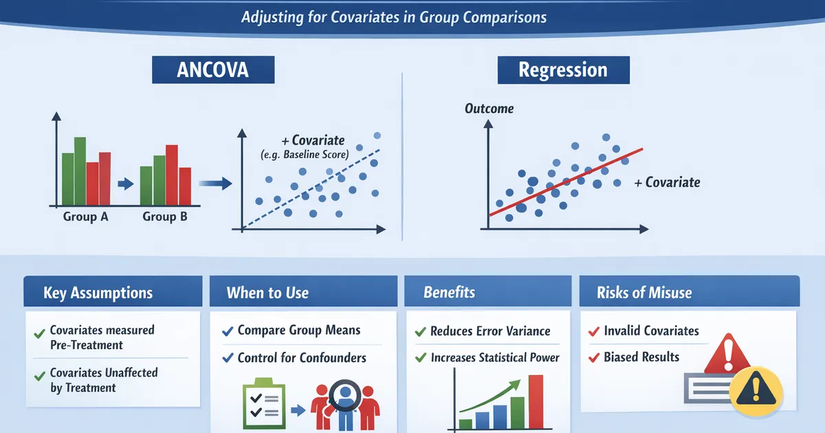
- •ANCOVA and regression adjustment are mathematically equivalent
- •Covariates must be measured before treatment and unaffected by treatment
- •Adjusting for baseline values increases power by reducing error variance
- •Violated assumptions can introduce bias rather than remove it
TL;DR
ANCOVA (Analysis of Covariance) and regression adjustment are mathematically identical methods for controlling covariates when comparing groups. Adjusting for pre-treatment covariates that correlate with the outcome increases power and corrects for baseline imbalances. The critical requirement: covariates must be measured before treatment and be unaffected by treatment. Adjusting for post-treatment variables introduces bias.
Why Adjust for Covariates?
Reduce Error Variance
If a covariate (like baseline score) correlates with the outcome, adjusting for it removes predictable variation, reducing error variance and increasing power.
import numpy as np
from scipy import stats
import statsmodels.api as sm
import pandas as pd

np.random.seed(42)

# Example: Testing an intervention
# Subjects have different baseline abilities (covariate)
n = 50
baseline = np.random.normal(100, 15, n * 2)  # Pre-treatment baseline

# Treatment assigned randomly
treatment = np.array([0] * n + [1] * n)

# Outcome depends on baseline + treatment effect + noise
# True treatment effect = 5
outcome = baseline + treatment * 5 + np.random.normal(0, 10, n * 2)

df = pd.DataFrame({
    'baseline': baseline,
    'treatment': treatment,
    'outcome': outcome
})

# Without adjustment
_, p_unadj = stats.ttest_ind(df[df['treatment']==0]['outcome'],
                              df[df['treatment']==1]['outcome'])

# With adjustment (ANCOVA)
model = sm.OLS.from_formula('outcome ~ treatment + baseline', data=df).fit()
p_adj = model.pvalues['treatment']

print(f"Without covariate adjustment: p = {p_unadj:.4f}")
print(f"With covariate adjustment: p = {p_adj:.4f}")
# Adjusted test is more powerful because baseline explains variance
Correct for Baseline Imbalance
Even with randomization, groups may differ on baseline characteristics. Adjustment corrects for these chance imbalances.
# Example: Imbalanced baseline (by chance)
df_imbalanced = df.copy()
# Imagine treatment group happened to have higher baseline
df_imbalanced.loc[df_imbalanced['treatment']==1, 'baseline'] += 5

# Unadjusted analysis is biased
unadj_means = df_imbalanced.groupby('treatment')['outcome'].mean()
print(f"\nUnadjusted means: Control={unadj_means[0]:.1f}, Treatment={unadj_means[1]:.1f}")
print(f"Unadjusted difference: {unadj_means[1] - unadj_means[0]:.1f}")

# Adjusted analysis removes baseline bias
model_adj = sm.OLS.from_formula('outcome ~ treatment + baseline',
                                 data=df_imbalanced).fit()
print(f"Adjusted treatment effect: {model_adj.params['treatment']:.1f}")
ANCOVA Model
ANCOVA models the outcome as:
Where:
- = grand mean
- = effect of group i
- = slope for covariate X
- = centered covariate
- = error
Python Implementation
import statsmodels.formula.api as smf

def ancova(df, outcome, group, covariate):
    """
    ANCOVA: Compare groups adjusting for covariate.
    """
    formula = f'{outcome} ~ C({group}) + {covariate}'
    model = smf.ols(formula, data=df).fit()

    # Adjusted means
    covariate_mean = df[covariate].mean()
    group_effects = model.params.filter(like=group)

    return {
        'model': model,
        'treatment_effect': model.params[f'C({group})[T.1]'],
        'covariate_slope': model.params[covariate],
        'p_value': model.pvalues[f'C({group})[T.1]'],
        'r_squared': model.rsquared
    }


result = ancova(df, 'outcome', 'treatment', 'baseline')
print(f"Treatment effect (adjusted): {result['treatment_effect']:.2f}")
print(f"Baseline slope: {result['covariate_slope']:.2f}")
print(f"P-value: {result['p_value']:.4f}")
print(f"R²: {result['r_squared']:.3f}")
R Implementation
# ANCOVA
model <- aov(outcome ~ treatment + baseline, data = df)
summary(model)

# Or using lm
model <- lm(outcome ~ treatment + baseline, data = df)
summary(model)

# Adjusted means
library(emmeans)
emmeans(model, ~ treatment)
Critical Assumptions
1. Covariate Measured Before Treatment
The covariate must be measured before treatment assignment or be unaffected by treatment.
Good: Baseline score, demographics, pre-treatment behavior Bad: Post-treatment mediator, variable affected by treatment
# WRONG: Adjusting for post-treatment variable
# This introduces collider bias

# Correct: Only adjust for pre-treatment variables
pre_treatment_covariates = ['baseline_score', 'age', 'prior_engagement']
2. Homogeneity of Regression Slopes
The relationship between covariate and outcome should be the same in all groups.
def test_homogeneity_of_slopes(df, outcome, group, covariate):
    """
    Test whether covariate slope differs by group.
    """
    # Model with interaction
    formula_interaction = f'{outcome} ~ C({group}) * {covariate}'
    model_int = smf.ols(formula_interaction, data=df).fit()

    # Test interaction term
    interaction_term = f'C({group})[T.1]:{covariate}'
    p_interaction = model_int.pvalues[interaction_term]

    return {
        'interaction_p': p_interaction,
        'slopes_equal': p_interaction > 0.05,
        'model': model_int
    }


# Check assumption
homog = test_homogeneity_of_slopes(df, 'outcome', 'treatment', 'baseline')
print(f"Interaction p-value: {homog['interaction_p']:.4f}")
print(f"Slopes appear equal: {homog['slopes_equal']}")
3. Covariate-Treatment Independence (Randomization)
In randomized experiments, treatment should be independent of covariates by design. If not (observational data), additional assumptions are needed.
ANCOVA vs. Change Scores
Two common approaches for pre-post designs:
ANCOVA Approach
Model post-treatment score adjusting for baseline:
Change Score Approach
Model change from baseline:
Which Is Better?
def compare_ancova_vs_change(df, baseline_col, outcome_col, treatment_col):
    """
    Compare ANCOVA and change score approaches.
    """
    # ANCOVA
    model_ancova = smf.ols(f'{outcome_col} ~ {treatment_col} + {baseline_col}',
                           data=df).fit()

    # Change score
    df = df.copy()
    df['change'] = df[outcome_col] - df[baseline_col]
    model_change = smf.ols(f'change ~ {treatment_col}', data=df).fit()

    return {
        'ancova_effect': model_ancova.params[treatment_col],
        'ancova_se': model_ancova.bse[treatment_col],
        'ancova_p': model_ancova.pvalues[treatment_col],
        'change_effect': model_change.params[treatment_col],
        'change_se': model_change.bse[treatment_col],
        'change_p': model_change.pvalues[treatment_col]
    }


comparison = compare_ancova_vs_change(df, 'baseline', 'outcome', 'treatment')
print("ANCOVA vs. Change Score:")
print(f"  ANCOVA: effect = {comparison['ancova_effect']:.2f}, "
      f"SE = {comparison['ancova_se']:.2f}, p = {comparison['ancova_p']:.4f}")
print(f"  Change: effect = {comparison['change_effect']:.2f}, "
      f"SE = {comparison['change_se']:.2f}, p = {comparison['change_p']:.4f}")
Conclusion: ANCOVA is generally more efficient (smaller SE) and handles regression to the mean better. Use ANCOVA unless you have specific reasons for change scores.
Multiple Covariates
Adjust for multiple pre-treatment variables:
def ancova_multiple_covariates(df, outcome, group, covariates):
    """
    ANCOVA with multiple covariates.
    """
    covariate_terms = ' + '.join(covariates)
    formula = f'{outcome} ~ C({group}) + {covariate_terms}'
    model = smf.ols(formula, data=df).fit()

    return model


# Example with multiple covariates
df['age'] = np.random.normal(35, 10, len(df))
df['prior_usage'] = np.random.exponential(10, len(df))

model = ancova_multiple_covariates(df, 'outcome', 'treatment',
                                    ['baseline', 'age', 'prior_usage'])
print(model.summary().tables[1])
Adjusted Means (EMMs)
Report estimated marginal means (adjusted for covariates) rather than raw group means:
def estimated_marginal_means(model, df, group_col, covariate_cols):
    """
    Calculate adjusted means at average covariate values.
    """
    # Create prediction data at mean covariate values
    groups = df[group_col].unique()
    emms = {}

    for group in groups:
        pred_data = {group_col: [group]}
        for cov in covariate_cols:
            pred_data[cov] = [df[cov].mean()]
        pred_df = pd.DataFrame(pred_data)

        emm = model.predict(pred_df)[0]
        emms[group] = emm

    return emms


# Calculate EMMs
from statsmodels.formula.api import ols
model = ols('outcome ~ C(treatment) + baseline', data=df).fit()
emms = estimated_marginal_means(model, df, 'treatment', ['baseline'])
print(f"Estimated marginal means:")
for group, emm in emms.items():
    print(f"  Treatment {group}: {emm:.2f}")
Common Mistakes
Adjusting for Post-Treatment Variables
Don't adjust for variables measured after treatment or affected by treatment—this introduces bias.
Adjusting for Colliders
A collider is affected by both treatment and outcome. Adjusting for it creates spurious associations.
Over-Adjustment
Adding too many covariates can increase variance and reduce power. Include only covariates that correlate with the outcome.
Ignoring Violated Assumptions
If slopes differ by group (significant interaction), standard ANCOVA is misleading. Either stratify or model the interaction.
Related Methods
- Comparing More Than Two Groups — The pillar guide
- CUPED and Variance Reduction — Related technique for experiments
- Linear Regression Diagnostics — Checking regression assumptions
Key Takeaway
ANCOVA and regression adjustment are equivalent methods for controlling covariates in group comparisons. The key is that covariates must be pre-treatment and unaffected by treatment. When this holds, adjustment increases power and reduces bias from baseline imbalances. When violated, adjustment can introduce bias rather than remove it.
References
- https://www.jstor.org/stable/2529685
- https://www.jstor.org/stable/2983904
- Senn, S. (2006). Change from baseline and analysis of covariance revisited. *Statistics in Medicine*, 25(24), 4334-4344.
- Cochran, W. G. (1957). Analysis of covariance: its nature and uses. *Biometrics*, 13(3), 261-281.
- Van Breukelen, G. J. (2006). ANCOVA versus change from baseline: more power in randomized studies, more bias in nonrandomized studies. *Journal of Clinical Epidemiology*, 59(9), 920-925.
Frequently Asked Questions
When should I adjust for covariates?
Does covariate adjustment always help?
Is ANCOVA different from regression?
Key Takeaway
ANCOVA and regression adjustment are equivalent methods for controlling covariates in group comparisons. The key is that covariates must be pre-treatment and unaffected by treatment. When this holds, adjustment increases power and reduces bias from baseline imbalances. When violated, adjustment can introduce bias.