Contents
Bootstrap Confidence Intervals for Difference in Means
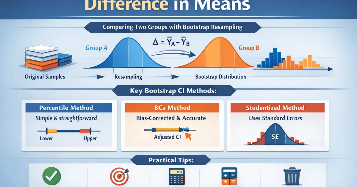
How to use bootstrap resampling to construct confidence intervals for comparing two groups. Covers percentile, BCa, and studentized methods with practical guidance.
Quick Hits
- •Bootstrap makes no distributional assumptions—it works for any statistic
- •Percentile method is simplest; BCa is more accurate for skewed data
- •10,000 bootstrap samples is standard; use more for p-values
- •Bootstrap estimates sampling variability, not bias—garbage in, garbage out
TL;DR
Bootstrap resampling constructs confidence intervals by repeatedly sampling from your data with replacement, computing your statistic each time, and using the distribution of results for inference. No distributional assumptions needed. The percentile method takes the 2.5th and 97.5th percentiles of bootstrap statistics. BCa adjusts for bias and skewness. With enough resamples (10,000+), bootstrap gives reliable intervals for virtually any statistic.
The Bootstrap Principle
Your sample is your best estimate of the population. Resampling from your sample (with replacement) simulates what would happen if you could resample from the population.
import numpy as np
from scipy import stats

def basic_bootstrap(group1, group2, statistic_func, n_bootstrap=10000):
    """
    Basic bootstrap for any statistic comparing two groups.

    statistic_func: function(g1, g2) -> scalar
    """
    # Observed statistic
    observed = statistic_func(group1, group2)

    # Bootstrap distribution
    boot_stats = []
    for _ in range(n_bootstrap):
        # Resample each group independently
        boot1 = np.random.choice(group1, size=len(group1), replace=True)
        boot2 = np.random.choice(group2, size=len(group2), replace=True)
        boot_stats.append(statistic_func(boot1, boot2))

    return observed, np.array(boot_stats)


# Example: difference in means
np.random.seed(42)
control = np.random.exponential(10, 100)
treatment = np.random.exponential(12, 100)

mean_diff = lambda g1, g2: np.mean(g2) - np.mean(g1)
observed, boot_dist = basic_bootstrap(control, treatment, mean_diff)

print(f"Observed difference: {observed:.2f}")
print(f"Bootstrap mean: {np.mean(boot_dist):.2f}")
print(f"Bootstrap SE: {np.std(boot_dist):.2f}")
Method 1: Percentile Bootstrap
The simplest method: take percentiles of the bootstrap distribution.
def percentile_ci(boot_stats, alpha=0.05):
    """
    Percentile bootstrap confidence interval.
    """
    lower = np.percentile(boot_stats, 100 * alpha / 2)
    upper = np.percentile(boot_stats, 100 * (1 - alpha / 2))
    return lower, upper


ci = percentile_ci(boot_dist)
print(f"95% Percentile CI: [{ci[0]:.2f}, {ci[1]:.2f}]")
When It Works
- Symmetric distributions
- Moderate sample sizes
- Statistics close to normally distributed
When It Struggles
- Skewed bootstrap distributions
- Bias in the bootstrap estimate
- Small samples
Method 2: BCa Bootstrap (Bias-Corrected and Accelerated)
Adjusts for bias and skewness in the bootstrap distribution.
from scipy.stats import norm

def bca_ci(data1, data2, boot_stats, observed_stat, alpha=0.05):
    """
    BCa (bias-corrected and accelerated) bootstrap CI.
    """
    n_boot = len(boot_stats)

    # Bias correction: proportion of bootstrap stats below observed
    z0 = norm.ppf(np.mean(boot_stats < observed_stat))

    # Acceleration: based on jackknife influence values
    combined = np.concatenate([data1, data2])
    n = len(combined)

    # Jackknife estimates (leaving out each observation)
    jackknife_stats = []
    for i in range(len(data1)):
        jack_data1 = np.delete(data1, i)
        jack_stat = np.mean(data2) - np.mean(jack_data1)
        jackknife_stats.append(jack_stat)
    for i in range(len(data2)):
        jack_data2 = np.delete(data2, i)
        jack_stat = np.mean(jack_data2) - np.mean(data1)
        jackknife_stats.append(jack_stat)

    jackknife_stats = np.array(jackknife_stats)
    jack_mean = np.mean(jackknife_stats)

    # Acceleration factor
    numerator = np.sum((jack_mean - jackknife_stats)**3)
    denominator = 6 * (np.sum((jack_mean - jackknife_stats)**2))**(3/2)

    if denominator == 0:
        a = 0
    else:
        a = numerator / denominator

    # Adjusted percentiles
    z_alpha_lower = norm.ppf(alpha / 2)
    z_alpha_upper = norm.ppf(1 - alpha / 2)

    alpha1 = norm.cdf(z0 + (z0 + z_alpha_lower) / (1 - a * (z0 + z_alpha_lower)))
    alpha2 = norm.cdf(z0 + (z0 + z_alpha_upper) / (1 - a * (z0 + z_alpha_upper)))

    lower = np.percentile(boot_stats, 100 * alpha1)
    upper = np.percentile(boot_stats, 100 * alpha2)

    return lower, upper


bca = bca_ci(control, treatment, boot_dist, observed)
print(f"95% BCa CI: [{bca[0]:.2f}, {bca[1]:.2f}]")
Using scipy.stats.bootstrap
from scipy.stats import bootstrap

def statistic(x, y, axis):
    return np.mean(y, axis=axis) - np.mean(x, axis=axis)

result = bootstrap((control, treatment), statistic,
                   n_resamples=10000, method='BCa',
                   confidence_level=0.95)

print(f"95% BCa CI (scipy): [{result.confidence_interval.low:.2f}, "
      f"{result.confidence_interval.high:.2f}]")
Method 3: Studentized (Bootstrap-t) Bootstrap
Uses pivotal quantity for better theoretical properties.
def studentized_bootstrap(group1, group2, n_bootstrap=10000, alpha=0.05):
    """
    Studentized (bootstrap-t) confidence interval.
    """
    # Observed statistic and SE
    observed_diff = np.mean(group2) - np.mean(group1)
    observed_se = np.sqrt(np.var(group1, ddof=1)/len(group1) +
                          np.var(group2, ddof=1)/len(group2))

    # Bootstrap t-statistics
    t_stats = []
    for _ in range(n_bootstrap):
        boot1 = np.random.choice(group1, size=len(group1), replace=True)
        boot2 = np.random.choice(group2, size=len(group2), replace=True)

        boot_diff = np.mean(boot2) - np.mean(boot1)
        boot_se = np.sqrt(np.var(boot1, ddof=1)/len(boot1) +
                         np.var(boot2, ddof=1)/len(boot2))

        t_stats.append((boot_diff - observed_diff) / boot_se)

    t_stats = np.array(t_stats)

    # Percentiles of t-distribution
    t_lower = np.percentile(t_stats, 100 * (1 - alpha/2))
    t_upper = np.percentile(t_stats, 100 * alpha/2)

    # CI using observed SE
    ci_lower = observed_diff - t_lower * observed_se
    ci_upper = observed_diff - t_upper * observed_se

    return ci_lower, ci_upper


stud_ci = studentized_bootstrap(control, treatment)
print(f"95% Studentized CI: [{stud_ci[0]:.2f}, {stud_ci[1]:.2f}]")
Comparison of Methods
| Method | Pros | Cons |
|---|---|---|
| Percentile | Simple, intuitive | Biased for skewed distributions |
| BCa | Adjusts for bias and skewness | More complex, needs jackknife |
| Studentized | Best theoretical properties | Requires SE estimation, nested bootstrap |
Bootstrap P-Values
Two approaches: permutation-based and direct.
Permutation Test
def permutation_pvalue(group1, group2, n_permutations=10000):
    """
    Permutation test p-value for difference in means.
    """
    observed_diff = np.mean(group2) - np.mean(group1)

    combined = np.concatenate([group1, group2])
    n1 = len(group1)

    # Permutation distribution
    perm_diffs = []
    for _ in range(n_permutations):
        np.random.shuffle(combined)
        perm_diff = np.mean(combined[n1:]) - np.mean(combined[:n1])
        perm_diffs.append(perm_diff)

    perm_diffs = np.array(perm_diffs)

    # Two-sided p-value
    p_value = np.mean(np.abs(perm_diffs) >= np.abs(observed_diff))

    return p_value


p_val = permutation_pvalue(control, treatment)
print(f"Permutation p-value: {p_val:.4f}")
Bootstrap-Based P-Value
def bootstrap_pvalue(group1, group2, n_bootstrap=10000):
    """
    Bootstrap p-value using shift to null hypothesis.
    """
    observed_diff = np.mean(group2) - np.mean(group1)

    # Shift treatment to have same mean as control (null hypothesis)
    group2_null = group2 - np.mean(group2) + np.mean(group1)

    # Bootstrap under null
    null_diffs = []
    for _ in range(n_bootstrap):
        boot1 = np.random.choice(group1, size=len(group1), replace=True)
        boot2 = np.random.choice(group2_null, size=len(group2_null), replace=True)
        null_diffs.append(np.mean(boot2) - np.mean(boot1))

    null_diffs = np.array(null_diffs)

    # Two-sided p-value
    p_value = np.mean(np.abs(null_diffs) >= np.abs(observed_diff))

    return p_value


p_val = bootstrap_pvalue(control, treatment)
print(f"Bootstrap p-value: {p_val:.4f}")
Complete Bootstrap Analysis
def full_bootstrap_analysis(group1, group2, n_bootstrap=10000, alpha=0.05):
    """
    Complete bootstrap analysis for comparing two groups.
    """
    # Observed statistics
    mean1, mean2 = np.mean(group1), np.mean(group2)
    diff = mean2 - mean1

    # Bootstrap
    boot_diffs = []
    for _ in range(n_bootstrap):
        boot1 = np.random.choice(group1, size=len(group1), replace=True)
        boot2 = np.random.choice(group2, size=len(group2), replace=True)
        boot_diffs.append(np.mean(boot2) - np.mean(boot1))

    boot_diffs = np.array(boot_diffs)

    # Confidence intervals
    ci_percentile = (np.percentile(boot_diffs, 100 * alpha/2),
                     np.percentile(boot_diffs, 100 * (1 - alpha/2)))

    # Bootstrap SE
    boot_se = np.std(boot_diffs)

    # P-value via permutation
    combined = np.concatenate([group1, group2])
    n1 = len(group1)
    perm_diffs = []
    for _ in range(n_bootstrap):
        np.random.shuffle(combined)
        perm_diffs.append(np.mean(combined[n1:]) - np.mean(combined[:n1]))
    p_value = np.mean(np.abs(perm_diffs) >= np.abs(diff))

    return {
        'group1_mean': mean1,
        'group2_mean': mean2,
        'difference': diff,
        'bootstrap_se': boot_se,
        'ci_95': ci_percentile,
        'p_value': p_value,
        'n_bootstrap': n_bootstrap
    }


result = full_bootstrap_analysis(control, treatment)
print(f"Group 1 mean: {result['group1_mean']:.2f}")
print(f"Group 2 mean: {result['group2_mean']:.2f}")
print(f"Difference: {result['difference']:.2f}")
print(f"Bootstrap SE: {result['bootstrap_se']:.2f}")
print(f"95% CI: [{result['ci_95'][0]:.2f}, {result['ci_95'][1]:.2f}]")
print(f"P-value: {result['p_value']:.4f}")
How Many Bootstrap Samples?
| Purpose | Recommended B |
|---|---|
| Quick exploration | 1,000 |
| Standard CI | 10,000 |
| BCa CI | 10,000+ |
| Precise p-values | 50,000-100,000 |
| Publication | 10,000-50,000 |
Rule: Bootstrap SE of a percentile decreases as . Doubling precision requires samples.
Limitations
What Bootstrap CAN'T Do
- Fix bias: If your sample is biased, bootstrap intervals will be centered on the wrong value
- Fix small samples: With n=10, bootstrap has limited information to work with
- Handle dependent data: Standard bootstrap assumes independence; use block bootstrap for time series
- Extrapolate: Can't estimate quantities outside the range of your data
When to Be Cautious
- Very small samples (n < 20)
- Discrete data with few unique values
- Heavy tails where extremes dominate
- Correlated observations
Related Methods
- Picking the Right Test to Compare Two Groups — Complete decision framework
- Non-Normal Metrics: Bootstrap, Mann-Whitney, and Log Transforms — Broader context
- Delta Method vs. Bootstrap — Alternative approaches
Key Takeaway
Bootstrap confidence intervals let you quantify uncertainty for any statistic without distributional assumptions. The percentile method is your default for simplicity; BCa handles skewness better. With 10,000+ resamples, bootstrap gives reliable intervals for most practical situations. Just remember: bootstrap estimates sampling variability, not bias—your sample still needs to be representative.
References
- https://www.jstor.org/stable/2289144
- https://www.stat.cmu.edu/~cshalizi/402/lectures/08-bootstrap/lecture-08.pdf
- Efron, B., & Tibshirani, R. J. (1993). *An Introduction to the Bootstrap*. Chapman & Hall/CRC.
- DiCiccio, T. J., & Efron, B. (1996). Bootstrap confidence intervals. *Statistical Science*, 11(3), 189-228.
- Davison, A. C., & Hinkley, D. V. (1997). *Bootstrap Methods and Their Application*. Cambridge University Press.
Frequently Asked Questions
How many bootstrap samples do I need?
Which bootstrap CI method should I use?
Can bootstrap fix biased samples?
Key Takeaway
Bootstrap confidence intervals let you quantify uncertainty for any statistic without distributional assumptions. The percentile method is your default; BCa handles skewness better. With 10,000+ resamples, bootstrap gives reliable intervals for most practical situations.