Contents
Alternatives to Cox: Accelerated Failure Time and Other Models
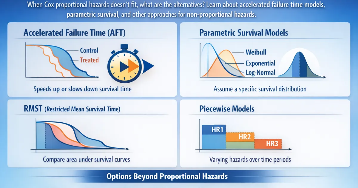
When Cox proportional hazards doesn't fit, what are the alternatives? Learn about accelerated failure time models, parametric survival, and other approaches for non-proportional hazards.
Quick Hits
- •Cox assumes proportional hazards - when that fails, consider alternatives
- •AFT models: treatment 'speeds up' or 'slows down' time to event
- •Parametric models (Weibull, exponential) assume a distribution for survival times
- •RMST: compare area under survival curves, no distributional assumptions
- •Piecewise models: different hazard ratios for different time periods
TL;DR
When Cox proportional hazards doesn't fit—because curves cross, effects change over time, or hazard ratios aren't interpretable—consider alternatives. Accelerated failure time (AFT) models express effects as time ratios ("treatment doubles survival time"). Parametric models (Weibull, log-normal) are efficient but require correct distributional assumptions. Restricted mean survival time (RMST) needs no assumptions but requires choosing a time horizon. This guide covers when and how to use each.
Why Look Beyond Cox?
Cox Regression Requires
- Proportional hazards: HR constant over time
- Interpretable hazard ratios: HR as the effect measure makes sense
When These Fail
- Curves cross: HR positive early, negative late (or vice versa)
- Effect wears off: Treatment helps initially, fades over time
- Time ratio is more intuitive: "Lives twice as long" vs "hazard halved"
- Prediction is goal: Cox doesn't easily predict survival times
Accelerated Failure Time (AFT) Models
The Concept
AFT models express covariate effects as speeding up or slowing down time:
Interpretation: Covariates multiply survival time.
If (log scale), then :
- Treatment extends survival time by 65%
- Someone who would survive 100 days survives 165 days
Time Ratio vs. Hazard Ratio
| Cox | AFT |
|---|---|
| HR = 0.6 | Time Ratio = 1.67 |
| "40% lower hazard" | "67% longer survival time" |
| Hazard reduced | Time extended |
These are related but not interchangeable. except for specific distributions.
Common AFT Distributions
| Distribution | Hazard Shape | When to Use |
|---|---|---|
| Exponential | Constant | Hazard doesn't change over time |
| Weibull | Monotonic | Hazard always increasing or always decreasing |
| Log-logistic | Unimodal/Monotonic | Hazard peaks then decreases |
| Log-normal | Unimodal | Heavy right tail |
| Generalized Gamma | Flexible | Encompasses many shapes |
Code: AFT Models
from lifelines import WeibullAFTFitter, LogNormalAFTFitter, LogLogisticAFTFitter


def fit_aft_models(data, time_col, event_col, covariates):
    """
    Fit multiple AFT models and compare.
    """
    model_data = data[[time_col, event_col] + covariates]

    results = {}

    # Weibull AFT
    weibull = WeibullAFTFitter()
    weibull.fit(model_data, duration_col=time_col, event_col=event_col)
    results['weibull'] = {
        'model': weibull,
        'aic': weibull.AIC_,
        'time_ratios': np.exp(weibull.params_['mu_'])
    }

    # Log-normal AFT
    lognormal = LogNormalAFTFitter()
    lognormal.fit(model_data, duration_col=time_col, event_col=event_col)
    results['lognormal'] = {
        'model': lognormal,
        'aic': lognormal.AIC_,
        'time_ratios': np.exp(lognormal.params_['mu_'])
    }

    # Log-logistic AFT
    loglogistic = LogLogisticAFTFitter()
    loglogistic.fit(model_data, duration_col=time_col, event_col=event_col)
    results['loglogistic'] = {
        'model': loglogistic,
        'aic': loglogistic.AIC_,
        'time_ratios': np.exp(loglogistic.params_['alpha_'])
    }

    # Compare AIC
    comparison = pd.DataFrame({
        'Model': ['Weibull', 'Log-Normal', 'Log-Logistic'],
        'AIC': [results['weibull']['aic'],
                results['lognormal']['aic'],
                results['loglogistic']['aic']]
    }).sort_values('AIC')

    results['comparison'] = comparison

    return results
library(survival)
library(flexsurv)

# Weibull AFT
weibull_aft <- survreg(Surv(time, event) ~ treatment + age,
                        data = data, dist = "weibull")

# Log-normal AFT
lognormal_aft <- survreg(Surv(time, event) ~ treatment + age,
                          data = data, dist = "lognormal")

# Compare AIC
AIC(weibull_aft, lognormal_aft)

# Time ratio (acceleration factor)
exp(coef(weibull_aft))
Parametric Survival Models
The Approach
Specify a distribution for survival times, estimate parameters.
Where f is a known distributional form (Weibull, exponential, etc.) with parameters θ.
Advantages Over Cox
- Efficiency: More precise estimates if distribution is correct
- Prediction: Can predict survival times and probabilities
- Extrapolation: Can extrapolate beyond observed data (with caution)
- Interpretability: Parameters often have intuitive meaning
Disadvantages
- Misspecification: Wrong distribution → biased results
- Rigidity: Less flexible than non-parametric methods
- Requires choice: Must select a distribution
Choosing a Distribution
Method 1: Visual comparison to Kaplan-Meier
from lifelines import KaplanMeierFitter, WeibullFitter

# Fit KM
kmf = KaplanMeierFitter()
kmf.fit(data['time'], data['event'])

# Fit parametric
wf = WeibullFitter()
wf.fit(data['time'], data['event'])

# Plot both
ax = kmf.plot_survival_function(label='Kaplan-Meier')
wf.plot_survival_function(ax=ax, label='Weibull')
Method 2: AIC/BIC comparison
Fit multiple distributions, compare information criteria.
Method 3: Hazard shape
- Constant hazard → Exponential
- Monotonic (increasing or decreasing) → Weibull
- Peak then decline → Log-logistic or log-normal
Restricted Mean Survival Time (RMST)
The Concept
RMST is the area under the survival curve up to a time horizon :
Interpretation: Expected survival time restricted to .
Advantages
- No proportional hazards assumption
- Works when curves cross
- Interpretable: "X extra days of survival"
- Non-parametric: No distributional assumptions
Disadvantages
- Requires choosing : Results depend on time horizon
- Less efficient: Doesn't use full distributional information
- Not a full model: Doesn't model the whole survival curve
Code: RMST
from lifelines import restricted_mean_survival_time, KaplanMeierFitter


def compare_rmst(data, time_col, event_col, group_col, tau):
    """
    Compare RMST between groups.
    """
    groups = sorted(data[group_col].unique())
    results = {}

    for group in groups:
        mask = data[group_col] == group
        kmf = KaplanMeierFitter()
        kmf.fit(data.loc[mask, time_col], data.loc[mask, event_col])

        rmst = restricted_mean_survival_time(kmf, t=tau)
        results[group] = rmst

    diff = results[groups[1]] - results[groups[0]]

    return {
        'rmst_by_group': results,
        'difference': diff,
        'interpretation': f"Group {groups[1]} survives {diff:.1f} days longer on average (up to day {tau})"
    }
library(survRM2)

# Compare RMST between groups
rmst_result <- rmst2(
    data$time,
    data$event,
    data$treatment,
    tau = 180  # Time horizon
)

print(rmst_result)
Piecewise and Time-Varying Models
When Effects Change Over Time
If treatment helps early but not late (or vice versa), a single HR misleads.
Piecewise approach: Fit different HRs for different time periods.
from lifelines import CoxPHFitter
import pandas as pd

def piecewise_cox(data, time_col, event_col, covariate, cutpoints):
    """
    Fit piecewise Cox model with different HRs by period.
    """
    results = []
    prev_cut = 0

    for cut in cutpoints + [float('inf')]:
        # Filter to observations at risk in this period
        period_data = data[data[time_col] > prev_cut].copy()

        # Censor at end of period
        period_data['_time'] = np.minimum(period_data[time_col] - prev_cut, cut - prev_cut)
        period_data['_event'] = np.where(
            period_data[time_col] <= cut,
            period_data[event_col],
            0
        )

        if period_data['_event'].sum() > 5:  # Need events
            cph = CoxPHFitter()
            cph.fit(period_data[['_time', '_event', covariate]],
                    duration_col='_time', event_col='_event')

            hr = np.exp(cph.params_[covariate])
            results.append({
                'period': f'{prev_cut}-{cut}' if cut < float('inf') else f'{prev_cut}+',
                'HR': hr,
                'p_value': cph.summary['p'][covariate]
            })

        prev_cut = cut

    return pd.DataFrame(results)
Time-Varying Coefficients in Cox
Allow HR to change smoothly over time:
# Include interaction with log(time)
cph = CoxPHFitter()
cph.fit(data, duration_col='time', event_col='event',
        formula='treatment + treatment:np.log(time)')
Decision Framework: Which Model?
START: Survival data analysis
       ↓
QUESTION: Does proportional hazards hold?
├── Yes → Cox regression (standard)
└── No or Unsure → Continue
       ↓
QUESTION: What's more interpretable for your question?
├── Time ratios ("lives X times longer") → AFT model
├── Hazard still meaningful → Consider below
└── Neither → RMST
       ↓
QUESTION: Is parametric distribution appropriate?
├── Yes, and you know which → Parametric AFT/PH
├── Unsure → Compare distributions via AIC
└── No → Non-parametric alternatives
       ↓
QUESTION: Do effects change over time?
├── Yes, distinct periods → Piecewise model
├── Yes, gradual change → Time-varying coefficient
└── No → Single model
       ↓
QUESTION: What's your primary goal?
├── Prediction → Parametric models
├── Causal inference → Appropriate model + sensitivity
└── Description → RMST or KM comparison
Comparison Summary
| Method | Assumptions | Output | Best For |
|---|---|---|---|
| Cox PH | Proportional hazards | Hazard ratios | Standard survival regression |
| AFT (Weibull) | Distribution, PH variant | Time ratios | Time-scaling interpretation |
| AFT (Log-normal) | Distribution | Time ratios | Heavy-tailed data |
| RMST | None | Days gained | Non-PH, interpretable summary |
| Piecewise Cox | PH within periods | Period-specific HRs | Changing effects |
| KM + log-rank | Non-informative censoring | Curves, p-values | Descriptive comparison |
Related Methods
- Time-to-Event and Retention Analysis (Pillar) - Full survival framework
- Cox Proportional Hazards - Standard approach
- Log-Rank Test - Non-parametric comparison
- Hazard Ratio Interpretation - Understanding HRs
Key Takeaway
Cox regression is the default for survival analysis, but it's not the only option. When proportional hazards fails, consider AFT models (intuitive time ratios), parametric models (efficient if correctly specified), RMST (no assumptions, interpretable as "days gained"), or piecewise models (when effects change over time). Choose based on what makes your results interpretable and your assumptions defensible.
References
- https://doi.org/10.1177/0962280218772293
- https://doi.org/10.1002/sim.7977
- https://lifelines.readthedocs.io/en/latest/Survival%20Regression.html
- Royston, P., & Parmar, M. K. (2002). Flexible parametric proportional-hazards and proportional-odds models for censored survival data. *Statistics in Medicine*, 21(15), 2175-2197.
- Uno, H., Claggett, B., Tian, L., et al. (2014). Moving beyond the hazard ratio in quantifying the between-group difference in survival analysis. *Journal of Clinical Oncology*, 32(22), 2380-2385.
- Wei, L. J. (1992). The accelerated failure time model: a useful alternative to the Cox regression model in survival analysis. *Statistics in Medicine*, 11(14-15), 1871-1879.
Frequently Asked Questions
When should I use AFT instead of Cox?
What's the difference between parametric and semi-parametric models?
Which distribution should I use for parametric survival?
Key Takeaway
Cox regression isn't the only option for survival data. When proportional hazards fails, consider accelerated failure time models (interpretable time ratios), parametric models (efficiency if correctly specified), RMST (no assumptions needed), or piecewise/time-varying models. Choose based on interpretability, assumption fit, and your specific question.