Contents
Sequential Testing: How to Peek at P-Values Without Inflating False Positives
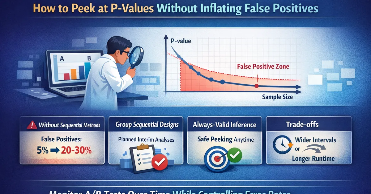
Learn how sequential testing methods let you monitor A/B test results as data accumulates while maintaining valid statistical guarantees. Covers group sequential designs, always-valid inference, and practical implementation.
Quick Hits
- •Peeking at results without sequential methods inflates false positives from 5% to 20-30%
- •Group sequential designs pre-specify analysis times and adjust significance thresholds
- •Always-valid inference lets you peek anytime while maintaining valid confidence intervals
- •The cost of peeking correctly is wider intervals or longer expected runtime
TL;DR
Classical hypothesis tests assume you analyze data once at a pre-specified time. If you peek at results repeatedly—which every product team does—your false positive rate inflates dramatically. Sequential testing methods let you monitor experiments as data arrives while maintaining valid statistical guarantees. The cost: slightly wider confidence intervals or longer maximum runtime.
The Peeking Problem
You launch an A/B test planned for two weeks. After three days, stakeholders ask "how's it looking?" You run the analysis. Treatment is up 8% with . Ship it?
If this was your planned analysis time, maybe. But if you planned to run two weeks and just happened to check early, that doesn't mean what you think.
Why Peeking Inflates False Positives
Classical p-values control the false positive rate at a single, pre-specified analysis time. Each additional peek is another opportunity to observe a spuriously significant result.
Think of it like coin flipping. The chance of flipping heads at least once in a single flip is 50%. But flip repeatedly? The chance of seeing heads at least once in 5 flips is 97%.
Similarly, check your experiment once at , and false positive rate is 5%. Check repeatedly? It compounds.
Simulation Evidence
import numpy as np
from scipy import stats

def simulate_peeking_inflation(n_simulations=10000, sample_size=5000, n_peeks=5):
    """
    Simulate A/A tests with peeking to measure false positive inflation.

    Returns:
        False positive rate across simulations
    """
    peek_points = np.linspace(sample_size // n_peeks, sample_size, n_peeks, dtype=int)
    false_positives = 0

    for _ in range(n_simulations):
        # Generate data from identical distributions (true null)
        control = np.random.normal(0, 1, sample_size)
        treatment = np.random.normal(0, 1, sample_size)  # Same distribution!

        for n in peek_points:
            _, p_value = stats.ttest_ind(control[:n], treatment[:n])
            if p_value < 0.05:
                false_positives += 1
                break  # Count as FP if ever significant

    return false_positives / n_simulations


# Run simulation
fp_rate = simulate_peeking_inflation(n_peeks=5)
print(f"False positive rate with 5 peeks: {fp_rate:.1%}")
# Typically ~20-30%, not 5%!
With 5 peeks, the false positive rate can reach 20-30%. With continuous monitoring, it approaches 100%—you'll eventually see "significance" by chance.
Solution 1: Group Sequential Designs
Group sequential designs pre-specify analysis times (called "looks") and adjust the significance threshold at each look to control overall false positive rate.
O'Brien-Fleming Boundaries
The O'Brien-Fleming approach uses very conservative thresholds early, becoming more liberal as the experiment progresses:
| Look | Cumulative Sample | Significance Threshold |
|---|---|---|
| 1 | 25% | 0.00005 |
| 2 | 50% | 0.0013 |
| 3 | 75% | 0.0085 |
| 4 | 100% | 0.041 |
Early significance requires overwhelming evidence. By the final look, the threshold is close to standard .
from scipy import stats
import numpy as np

def obrien_fleming_boundaries(n_looks, alpha=0.05):
    """
    Calculate O'Brien-Fleming spending function boundaries.

    Approximate boundaries using the spending function approach.
    """
    boundaries = []
    info_fractions = np.linspace(1/n_looks, 1, n_looks)

    for t in info_fractions:
        # O'Brien-Fleming spending function
        spent = 2 * (1 - stats.norm.cdf(stats.norm.ppf(1 - alpha/2) / np.sqrt(t)))
        z_boundary = stats.norm.ppf(1 - spent/2)
        boundaries.append({
            'info_fraction': t,
            'z_boundary': z_boundary,
            'p_threshold': 2 * (1 - stats.norm.cdf(z_boundary))
        })

    return boundaries


boundaries = obrien_fleming_boundaries(n_looks=4)
for b in boundaries:
    print(f"At {b['info_fraction']:.0%} info: z={b['z_boundary']:.2f}, "
          f"p-threshold={b['p_threshold']:.5f}")
Pocock Boundaries
Pocock boundaries use equal significance thresholds at each look:
| Look | Significance Threshold |
|---|---|
| 1-4 | 0.0182 |
Simpler to explain but less efficient—you "spend" more early when data is sparse.
Python Implementation with statsmodels
from statsmodels.stats.stattools import omni_normtest
import statsmodels.stats.api as sms

# Using the statsmodels GroupSequential class (if available)
# Otherwise, implement boundaries manually:

def sequential_test(control, treatment, n_looks=4, spending='obrien_fleming'):
    """
    Run a group sequential test with pre-specified looks.
    """
    n = len(control)
    look_sizes = [n * (i+1) // n_looks for i in range(n_looks)]

    boundaries = obrien_fleming_boundaries(n_looks)

    for i, look_n in enumerate(look_sizes):
        c_sample = control[:look_n]
        t_sample = treatment[:look_n]

        stat, p_value = stats.ttest_ind(c_sample, t_sample)
        z = stats.norm.ppf(1 - p_value/2) if p_value < 1 else 0

        threshold = boundaries[i]['z_boundary']

        print(f"Look {i+1} (n={look_n}): z={abs(z):.3f}, threshold={threshold:.3f}")

        if abs(z) > threshold:
            return {
                'stopped_early': True,
                'look': i + 1,
                'p_value': p_value,
                'effect': np.mean(t_sample) - np.mean(c_sample)
            }

    return {
        'stopped_early': False,
        'look': n_looks,
        'p_value': p_value,
        'effect': np.mean(treatment) - np.mean(control)
    }
R Implementation
library(gsDesign)

# Create a group sequential design
design <- gsDesign(
  k = 4,              # 4 looks
  test.type = 2,      # Two-sided
  alpha = 0.05,
  beta = 0.2,         # 80% power
  sfu = "OF"          # O'Brien-Fleming spending
)

# View boundaries
print(design)

# Check at each look
# If z-statistic exceeds boundary, stop and reject
Solution 2: Always-Valid Inference
Group sequential designs require pre-specifying look times. What if you want to check anytime without a schedule?
Always-valid inference provides confidence sequences that remain valid no matter when or how often you look.
Confidence Sequences
A confidence sequence is a sequence of confidence intervals that, with probability , simultaneously contain the true parameter at all times.
import numpy as np

def confidence_sequence_mean(data, alpha=0.05):
    """
    Compute always-valid confidence sequence for the mean.

    Uses the mixture method with stitching.
    """
    n = len(data)
    if n < 2:
        return (-np.inf, np.inf)

    mean = np.mean(data)
    var = np.var(data, ddof=1)

    # Asymptotic confidence sequence width
    # Based on the law of iterated logarithm
    rho = 1  # mixture parameter
    width = np.sqrt(2 * var * (1 + 1/n) * (np.log(np.log(max(n, np.e))) + 0.72 + np.log(2/alpha)) / n)

    return (mean - width, mean + width)


def sequential_comparison(control, treatment, alpha=0.05):
    """
    Compare two groups using confidence sequences.

    Returns confidence sequence for the difference.
    """
    # Compute difference for each paired observation
    # Or use separate sequences for each group

    # For unpaired, use separate sequences
    cs_control = confidence_sequence_mean(control, alpha/2)
    cs_treatment = confidence_sequence_mean(treatment, alpha/2)

    # Difference bounds (conservative combination)
    diff_lower = (np.mean(treatment) - np.mean(control) -
                  (cs_treatment[1] - np.mean(treatment)) -
                  (np.mean(control) - cs_control[0]))
    diff_upper = (np.mean(treatment) - np.mean(control) +
                  (cs_treatment[1] - np.mean(treatment)) +
                  (np.mean(control) - cs_control[0]))

    return diff_lower, diff_upper
Key Property
At any time t, the confidence sequence either:
- Excludes zero → stop and declare significance
- Includes zero → continue (or stop for futility)
You never "spend" significance level by peeking—the intervals are calibrated to be valid at all times simultaneously.
The Cost
Always-valid intervals are wider than fixed-time intervals at any given sample size. You pay for the flexibility to stop anytime with less precision at each moment.
Solution 3: Bayesian Monitoring
Bayesian approaches sidestep the frequentist peeking problem because they make direct statements about parameter probabilities, not long-run error rates.
Bayesian A/B Testing
import numpy as np
from scipy import stats

def bayesian_ab_test(control_conversions, control_total,
                     treatment_conversions, treatment_total,
                     prior_alpha=1, prior_beta=1):
    """
    Bayesian comparison of two conversion rates.

    Uses Beta-Binomial conjugate model.
    Returns probability that treatment > control.
    """
    # Posterior distributions (Beta)
    control_alpha = prior_alpha + control_conversions
    control_beta = prior_beta + control_total - control_conversions

    treatment_alpha = prior_alpha + treatment_conversions
    treatment_beta = prior_beta + treatment_total - treatment_conversions

    # Monte Carlo estimate of P(treatment > control)
    n_samples = 100000
    control_samples = np.random.beta(control_alpha, control_beta, n_samples)
    treatment_samples = np.random.beta(treatment_alpha, treatment_beta, n_samples)

    prob_treatment_better = np.mean(treatment_samples > control_samples)

    return {
        'prob_treatment_better': prob_treatment_better,
        'prob_control_better': 1 - prob_treatment_better,
        'control_mean': control_alpha / (control_alpha + control_beta),
        'treatment_mean': treatment_alpha / (treatment_alpha + treatment_beta)
    }


# Example: Check at any time
result = bayesian_ab_test(
    control_conversions=500, control_total=10000,
    treatment_conversions=550, treatment_total=10000
)
print(f"P(treatment > control): {result['prob_treatment_better']:.1%}")
Stopping Rules
You can stop when:
- P(treatment better) > 0.95 → ship treatment
- P(control better) > 0.95 → keep control
- Neither after maximum sample → declare inconclusive
The Catch
While Bayesian credible intervals don't suffer from the peeking problem in the same way, decision rules based on posterior probabilities can still have frequentist operating characteristics you care about (false positive rate, power). Design your stopping rules with these in mind.
Choosing a Method
| Method | Pros | Cons |
|---|---|---|
| Group Sequential | Well-established theory, easy to explain | Must pre-specify look times |
| Always-Valid | Peek anytime, no schedule needed | Wider intervals, newer theory |
| Bayesian | Intuitive interpretation, natural stopping | Requires prior specification, frequentist properties need verification |
Practical Recommendation
For most product teams:
- If you'll definitely peek on a schedule: Use group sequential design with O'Brien-Fleming boundaries
- If you need flexibility: Use always-valid confidence sequences
- If your org is Bayesian-friendly: Use Bayesian monitoring with calibrated stopping rules
Any of these is dramatically better than pretending you won't peek.
Implementation Checklist
Before the Test
- Decide whether you'll use sequential testing
- Choose your method (group sequential, always-valid, Bayesian)
- Pre-specify analysis times (if group sequential)
- Set stopping rules for both efficacy and futility
- Document everything
During the Test
- Only analyze at pre-specified times (if group sequential)
- Use proper adjusted thresholds for significance
- Record all looks and decisions
After the Test
- Report using the sequential framework
- Don't back-calculate "what the p-value would have been" with fixed-horizon methods
Common Mistakes
Using Fixed-Horizon P-Values After Peeking
If you peeked, your p-value from a standard test is not valid. Report results using the sequential method you actually used.
Informal "Just Checking"
There's no such thing as just checking without consequences. Either commit to not looking, or use sequential methods.
Stopping for Futility Without Planning
Stopping because results "look flat" is itself a form of peeking. Pre-specify futility stopping rules if you want that option.
Ignoring the Confidence Interval
Even with sequential testing, focus on the confidence interval, not just significance. A significant result with wide intervals may not be actionable.
Related Methods
- A/B Testing Statistical Methods for Product Teams — Complete guide to A/B testing
- MDE and Sample Size: A Practical Guide — Planning your experiment duration
- Multiple Experiments: FDR vs. Bonferroni — Managing false discoveries across many tests
Frequently Asked Questions
Q: How much extra sample does sequential testing require? A: Maximum sample is typically 20-30% larger than fixed-horizon. But average sample is often lower because you stop early for large effects.
Q: Can I convert an existing test to sequential testing mid-experiment? A: No. The validity guarantees require planning before data collection. You can't retroactively apply sequential methods.
Q: What if I need to peek but my org doesn't support sequential testing? A: Document every look you take. Report your results with appropriate caveats. Advocate for proper sequential methods in future experiments.
Q: Is Bayesian testing really immune to peeking? A: Bayesian posterior probabilities don't have the same peeking problem. However, if you care about frequentist error rates (and you should for decision-making), your stopping rules still need calibration.
Key Takeaway
If you're going to peek at your A/B test results (and you probably are), use sequential testing methods that are designed for it. The alternative—pretending you didn't peek—leads to false positives that erode trust in your experimentation program. The cost of doing it right (slightly wider intervals or longer runtime) is far less than the cost of systematic false discoveries.
References
- https://arxiv.org/abs/1512.04922
- https://www.tandfonline.com/doi/abs/10.1080/01621459.1977.10479947
- Johari, R., Koomen, P., Pekelis, L., & Walsh, D. (2017). Peeking at A/B Tests: Why It Matters, and What to Do About It. *KDD '17*.
- Jennison, C., & Turnbull, B. W. (2000). *Group Sequential Methods with Applications to Clinical Trials*. Chapman & Hall/CRC.
- Howard, S. R., Ramdas, A., McAuliffe, J., & Sekhon, J. (2021). Time-uniform, nonparametric, nonasymptotic confidence sequences. *The Annals of Statistics*, 49(2), 1055-1080.
Frequently Asked Questions
How much does sequential testing cost in sample size?
Can I use sequential testing for any metric?
Should I always use sequential testing?
Key Takeaway
If you're going to peek at your A/B test results (and you probably are), use sequential testing methods that are designed for it. The alternative—pretending you didn't peek—leads to false positives that erode trust in your experimentation program.