Contents
Synthetic Control: Building a Counterfactual for Geo Tests
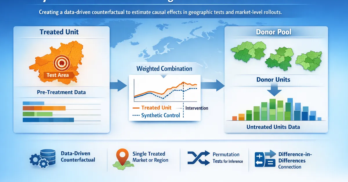
How the synthetic control method builds a data-driven counterfactual from donor units to estimate causal effects in geo tests and market-level rollouts.
Quick Hits
- •Synthetic control constructs a weighted combination of untreated units that matches the treated unit's pre-treatment trajectory, creating a data-driven counterfactual
- •It is ideal when you have a single treated unit (a market, region, or product line) and a pool of untreated units as donors
- •Pre-treatment fit quality is visually inspectable and quantifiable -- if the synthetic control can't match pre-treatment outcomes, the method shouldn't be trusted
- •Inference relies on permutation (placebo) tests rather than traditional p-values, making it valid even with small donor pools
- •Difference-in-differences is a special case of synthetic control where all donor units receive equal weight
TL;DR
When you roll out a change to a single market or region and want to know its causal impact, you need a counterfactual: what would have happened without the change? Synthetic control builds this counterfactual by finding a weighted combination of untreated markets that tracks the treated market's pre-treatment outcomes. The post-treatment divergence between the real market and its synthetic twin is your causal estimate. This post covers the method, implementation, inference, and practical considerations for product teams running geo tests.
The Problem: One Treated Unit, No Control Group
Product teams frequently launch changes at the market level: a new pricing model in a country, a marketing campaign in a region, a regulatory compliance feature in a jurisdiction. With only one treated unit, you cannot run a standard A/B test.
The naive approach -- comparing the treated market before and after the change -- confounds the treatment with time trends, seasonality, and concurrent events. A slightly better approach -- comparing to a single "similar" market -- assumes that market's trajectory would have matched the treated market's absent treatment (parallel trends). This assumption is often implausible.
Synthetic control improves on both by constructing an optimized counterfactual from multiple untreated markets.
How Synthetic Control Works
The Setup
- Treated unit: The single market or region that received the intervention.
- Donor pool: A set of untreated markets or regions that did not receive the intervention.
- Pre-treatment period: Time periods before the intervention.
- Post-treatment period: Time periods after the intervention.
The Algorithm
Synthetic control finds weights for the donor units such that:
Subject to: and (weights are non-negative and sum to one).
The synthetic control is the weighted average of donor outcomes using these optimized weights. In the post-treatment period, the causal effect estimate at time is:
The restriction to non-negative weights that sum to one prevents extrapolation. The synthetic control is always an interpolation of donor units, which is more credible than a model-based extrapolation.
Matching Predictors
In practice, you match not just on lagged outcomes but also on observable predictors (market size, demographic composition, baseline engagement levels). The optimizer minimizes a distance function that weights both pre-treatment outcomes and predictor match quality.
A Geo Test Example
Context: Your company launched a new checkout flow in Brazil. You want to estimate its effect on weekly revenue. Donor markets: Argentina, Mexico, Colombia, Chile, Peru, and five other Latin American markets.
Pre-treatment period: 52 weeks before the launch. Post-treatment period: 12 weeks after.
Steps:
- Assemble weekly revenue data for Brazil and all donor markets.
- Include predictors: market size (MAU), average order value, mobile share, and several pre-treatment lagged revenue values.
- Run the synthetic control optimizer to find weights.
- Result: Synthetic Brazil = 0.35 * Mexico + 0.28 * Colombia + 0.22 * Argentina + 0.15 * Chile.
- Plot real Brazil revenue against synthetic Brazil revenue.
- Pre-treatment: the two lines should track each other closely.
- Post-treatment: the gap between the lines is your causal estimate.
If real Brazil revenue is 8% above synthetic Brazil after launch, and this gap emerges precisely at the launch date, the new checkout flow plausibly caused an 8% revenue lift.
Inference: Placebo Tests
Traditional statistical inference does not apply directly to synthetic control because you have only one treated unit. Instead, inference relies on permutation (placebo) tests.
In-Space Placebos
Apply the synthetic control method to each donor unit in turn, pretending it was treated. This gives you a distribution of "placebo effects" -- the gaps you would see if the treatment had no effect.
If the treated unit's post-treatment gap is large relative to the donor gaps, the effect is unlikely due to chance. Formally, compute the ratio of post-treatment RMSPE to pre-treatment RMSPE for each unit. The treated unit's rank in this distribution provides a permutation-based p-value.
Example: If there are 10 donors and Brazil's gap is larger than all 10 placebo gaps, the p-value is . With 20 donors, the same result gives .
In-Time Placebos
Apply the method using a fake treatment date in the pre-treatment period. If the method produces a large gap at the fake date, the pre-treatment fit is fragile and the post-treatment estimate should not be trusted.
Key Assumptions
No Interference
Donor units must be unaffected by the treatment. If launching the checkout flow in Brazil diverted traffic from Mexico, Mexico's outcomes are contaminated, and the synthetic control is biased.
No Concurrent Events
No other intervention should affect the treated unit at the same time. If Brazil simultaneously launched a marketing campaign, the estimated effect combines both interventions.
Convex Hull
The treated unit's pre-treatment outcomes must lie within the convex hull of the donor pool. If Brazil's pre-treatment revenue is higher than all donors, no non-negative weighted combination can match it. In this case, synthetic control is not appropriate.
Stable Donor Characteristics
Donor units should not experience idiosyncratic shocks during the post-treatment period. If Colombia has an economic crisis shortly after Brazil's launch, the synthetic control is distorted.
Synthetic Control vs. Difference-in-Differences
Difference-in-differences (DiD) is the more familiar method. How do they compare?
| Feature | Synthetic Control | Difference-in-Differences |
|---|---|---|
| Weights | Data-driven, optimized | Equal (or pre-specified) |
| Parallel trends | Not required; pre-treatment match is directly visible | Required; often assumed, rarely verified |
| Number of treated units | Designed for one | Works best with many |
| Inference | Permutation-based | Standard (asymptotic) |
| Transparency | Weights and fit are visible | Assumption-based |
DiD is a special case of synthetic control where all donors get equal weight. If the equal-weight average already tracks the treated unit well, DiD is simpler and sufficient. If it does not, synthetic control is the upgrade.
When you have multiple treated units and a clear pre/post structure, DiD is often the better starting point. When you have a single treated unit and need a credible counterfactual, synthetic control is the tool.
Practical Considerations for Product Teams
Choosing the Donor Pool
Include markets that are plausibly similar to the treated market and unlikely to be affected by the treatment. Exclude markets that experienced their own shocks during the study period. More donors give the optimizer flexibility, but including irrelevant donors (markets with completely different trajectories) adds noise.
Pre-Treatment Fit Quality
The credibility of the entire method rests on how well the synthetic control matches the treated unit before treatment. If the pre-treatment fit is poor, the post-treatment comparison is meaningless. Aim for a root mean squared prediction error (RMSPE) that is small relative to the outcome's scale.
How Much Pre-Treatment Data?
More is generally better. With 52 weeks of pre-treatment data, seasonal patterns are captured. With only 4 weeks, transient fluctuations can produce spurious matches. A rule of thumb: use at least as many pre-treatment periods as you have donors, and capture full seasonal cycles.
Augmented Synthetic Control
Recent extensions (the augmented synthetic control method) combine synthetic control with an outcome model to reduce bias when the pre-treatment fit is imperfect. This is analogous to the doubly robust logic in propensity score matching: combining two approaches for robustness.
Common Pitfalls
Cherry-picking the donor pool. Including or excluding donors based on whether they produce the "right" result is p-hacking for synthetic control. Pre-specify your donor pool based on substantive criteria.
Poor pre-treatment fit. If the synthetic control does not track the treated unit before treatment, the gap after treatment is uninterpretable. Do not report results with bad pre-treatment fit.
Ignoring concurrent events. Always investigate what else happened to the treated market around the treatment date. A regulatory change, marketing push, or competitive entry can masquerade as a treatment effect.
Too few donors for inference. With only 3-4 donors, the permutation distribution has too few values to produce a meaningful p-value. Consider whether alternative methods like interrupted time series might be more appropriate.
When to Use Synthetic Control
Synthetic control is the right method when:
- You have a single (or few) treated units at an aggregate level (market, region, product line).
- You have a pool of untreated units with similar outcome trajectories.
- Pre-treatment data is available for a sufficient number of periods.
- No other intervention coincides with the treatment.
For user-level causal inference, consider propensity score matching or regression discontinuity. For the complete menu of causal inference methods, see our causal inference overview.
References
- https://web.stanford.edu/~jhain/Paper/JASA2010.pdf
- https://economics.mit.edu/sites/default/files/publications/Using%20Synthetic%20Controls.pdf
- https://matheusfacure.github.io/python-causality-handbook/15-Synthetic-Control.html
Frequently Asked Questions
How is synthetic control different from difference-in-differences?
How many donor units do I need?
Can I use synthetic control for user-level data?
Key Takeaway
Synthetic control builds a rigorous, data-driven counterfactual by weighting untreated units to match the treated unit's pre-treatment trajectory, making it the method of choice for estimating causal effects in geo tests and market-level rollouts with a single treated unit.