Contents
Seasonal Decomposition: Separating Signal from Calendar Effects
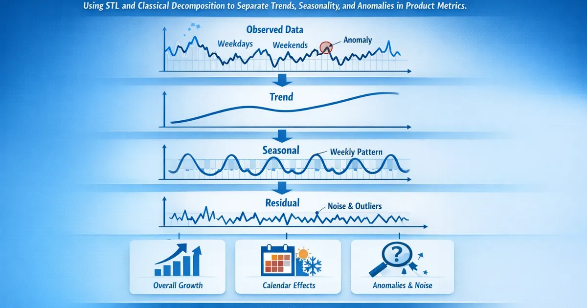
How to use STL and classical decomposition to separate trends, seasonality, and anomalies in product metrics.
Quick Hits
- •Most product metrics have day-of-week seasonality -- Monday DAU and Saturday DAU are structurally different
- •STL decomposition is the modern standard: robust to outliers and handles changing seasonality
- •Additive decomposition for constant seasonal swings, multiplicative when swings grow with the level
- •After decomposition, analyze the residual component for genuine anomalies and A/B test effects
- •Holiday effects are not seasonal -- they require separate modeling as one-off calendar events
TL;DR
Product metrics have calendar-driven patterns that confuse analysis. Monday engagement differs from Saturday engagement, December revenue differs from February revenue, and holiday weekends differ from regular weekends. Seasonal decomposition separates these predictable patterns from trends and genuine anomalies, letting you analyze each component independently. STL is the modern standard method, and this guide shows you how to apply it to product data.
Why Decomposition Matters for Product Analytics
Every time you compare this week's conversion rate to last week's, you are implicitly assuming the difference is meaningful. But what if conversion rates are always lower on weeks with holidays? What if engagement always dips mid-month? Without decomposition, you cannot distinguish a real change from a predictable calendar effect.
Decomposition answers three questions simultaneously:
- What is the underlying direction? (Trend component)
- What is the predictable pattern? (Seasonal component)
- What is genuinely unusual? (Residual component)
A stakeholder who sees a 5% revenue drop does not need to panic if the seasonal component explains a 6% dip and the trend is actually up 1%.
The Three Components
Trend ()
The long-term direction of the metric, stripped of seasonal fluctuations and noise. A smooth curve that shows whether your product is growing, plateauing, or declining.
For more on detecting and testing trends, see our guide on trend detection methods.
Seasonal ()
The repeating pattern at fixed intervals. For daily product data, the most common seasonal periods are:
- Weekly (period=7): Weekday vs. weekend differences in usage, engagement, and conversion
- Monthly (period~30): Paycheck cycles, billing cycles, end-of-month reporting pushes
- Annual (period=365): Holidays, back-to-school, summer slowdowns, Q4 spikes
The seasonal component repeats (approximately) every period. By definition, the seasonal effects sum to approximately zero over each cycle in an additive model, or to approximately 1 in a multiplicative model.
Residual ()
What remains after removing trend and seasonality. This is where genuine anomalies live -- product launches, outages, viral events, and A/B test effects. The residual should ideally look like uncorrelated noise. If patterns remain in the residual, your decomposition is incomplete.
Additive vs. Multiplicative Decomposition
Additive model:
The seasonal effect is a fixed amount. If DAU drops by 2,000 on weekends regardless of whether your average is 50,000 or 100,000, the relationship is additive.
Multiplicative model:
The seasonal effect is proportional. If revenue drops 15% on weekends whether your daily baseline is $100K or $500K, the relationship is multiplicative.
How to choose:
- Plot the data. Do seasonal swings grow with the level?
- If yes: multiplicative. If constant: additive.
- Shortcut: apply
log()to the data and use additive decomposition. Log-additive is mathematically equivalent to multiplicative decomposition.
Most revenue and transaction metrics are multiplicative. Most ratio metrics (conversion rates, retention rates) are additive or approximately so.
STL Decomposition: The Modern Standard
Why STL Over Classical Decomposition
Classical decomposition (moving average trend, simple seasonal averages) has serious limitations:
- The trend is undefined at the endpoints of the series
- The seasonal component is fixed -- it cannot evolve
- It is not robust to outliers
STL addresses all three:
- LOESS smoothing provides trend estimates all the way to the endpoints
- The seasonal component can change over time (controlled by a smoothing parameter)
- The
robust=Trueoption down-weights outliers iteratively
Implementation
from statsmodels.tsa.seasonal import STL
import pandas as pd

# Load daily metric data
daily_data = pd.read_csv("daily_dau.csv",
                          index_col="date",
                          parse_dates=True)

# STL with weekly seasonality
stl = STL(daily_data["dau"],
          period=7,
          seasonal=7,      # seasonal smoother span (odd number)
          trend=None,       # auto-select trend smoother
          robust=True)      # resist outliers
result = stl.fit()

# Access components
trend = result.trend
seasonal = result.seasonal
residual = result.resid
Key Parameters
period: The seasonal period. Use 7 for weekly seasonality in daily data, 12 for monthly seasonality in monthly data, 52 for weekly data with annual seasonality.
seasonal: The smoothing span for the seasonal component. Must be odd. Larger values produce a more stable seasonal pattern. Smaller values allow the pattern to change faster. Default is 7 for most implementations.
trend: The smoothing span for the trend. Larger values produce smoother trends. None selects automatically based on the period.
robust: When True, iteratively down-weights outliers. Always use True for product data, which frequently contains spikes and drops.
Handling Multiple Seasonal Periods
Daily product data often has both weekly and annual seasonality. Standard STL handles one period. For multiple periods, use MSTL (Multiple Seasonal-Trend decomposition using LOESS):
from statsmodels.tsa.seasonal import MSTL

# Decompose with weekly AND annual seasonality
mstl = MSTL(daily_data["revenue"],
             periods=[7, 365],
             stl_kwargs={"robust": True})
result = mstl.fit()

# Now has multiple seasonal components
weekly_seasonal = result.seasonal["period_7"]
annual_seasonal = result.seasonal["period_365"]
This is particularly important for metrics with strong holiday effects. Without the annual component, holiday spikes will appear in the residual and get flagged as anomalies.
Holiday and Special Event Effects
Holidays are not truly seasonal -- they do not repeat at perfectly regular intervals (Thanksgiving falls on different dates, Easter moves, promotions are irregular). Decomposition methods handle them imperfectly.
Approaches to holiday effects:
- Pre-processing: Remove known holiday periods before decomposition, then add them back as a separate component.
- Regression with dummy variables: Include holiday indicators in a regression model alongside trend and seasonal terms.
- Prophet: Facebook's Prophet model explicitly models holiday effects alongside trend and seasonality. See our guide on forecasting methods.
- Post-hoc flagging: Decompose without holiday adjustment, then manually flag residual spikes that correspond to known holidays.
For most product analytics work, approach 4 (decompose then flag) is sufficient. If holiday effects dominate your metric, use Prophet or a regression approach.
Using Decomposition Results
For Anomaly Detection
After decomposition, compute the residual's standard deviation. Flag observations where the residual exceeds or as anomalies:
import numpy as np

residual_std = np.std(residual)
anomalies = daily_data[np.abs(residual) > 3 * residual_std]
These are deviations from the expected pattern -- genuinely unusual observations that warrant investigation.
For Trend Reporting
Report the trend component to stakeholders instead of (or alongside) raw numbers. "DAU was 52,000 yesterday" is less informative than "DAU was 52,000, which is on trend -- the underlying trend is 51,800 and growing at 50 users per day."
For A/B Test Analysis
If your A/B test runs over multiple weeks, decompose the treatment group's metric and examine whether the residual during the test period is systematically positive or negative. This separates the test effect from seasonal patterns. For quasi-experimental designs, see our guides on interrupted time series and difference-in-differences.
For Forecasting
Decomposition components feed directly into forecasting. Project the trend forward, add the expected seasonal pattern, and construct prediction intervals from the residual's distribution. For formal forecasting methods, see our guide on ARIMA and Prophet.
Common Mistakes
Using too short a time series. To estimate weekly seasonality, you need at least 2-3 complete weeks. For annual seasonality, 2-3 complete years. With insufficient data, the seasonal component absorbs noise.
Ignoring the residual. Decomposition is not the end -- it is the beginning. Always check the residual for remaining patterns (look at its ACF). If the residual still shows autocorrelation, your decomposition missed something.
Applying additive decomposition to multiplicative data. If seasonal swings grow with the level, additive decomposition will systematically underestimate the seasonal effect during high periods and overestimate during low periods. Take the log first.
Treating decomposition as truth. Decomposition is a model, not a fact. The "trend" is defined by the smoothing parameters you chose. Different parameter settings produce different decompositions. Be transparent about your choices and check sensitivity.
References
- https://otexts.com/fpp3/decomposition.html
- https://www.statsmodels.org/stable/generated/statsmodels.tsa.seasonal.STL.html
- https://doi.org/10.6028/jres.090.015
- Cleveland, R. B., Cleveland, W. S., McRae, J. E., & Terpenning, I. (1990). STL: A seasonal-trend decomposition. *Journal of Official Statistics*, 6(1), 3-73.
- Hyndman, R. J., & Athanasopoulos, G. (2021). *Forecasting: Principles and Practice*, 3rd edition, Chapter 3. OTexts.
Frequently Asked Questions
How do I choose between additive and multiplicative decomposition?
Can I decompose data with multiple seasonal periods?
What if my seasonality changes over time?
Key Takeaway
Seasonal decomposition is the essential first step in time series analysis of product metrics. It separates your data into trend, seasonal, and residual components, letting you analyze each independently. STL is the recommended method for most product data because it handles outliers robustly and adapts to changing seasonal patterns.