Contents
Regression Discontinuity: When Thresholds Create Experiments
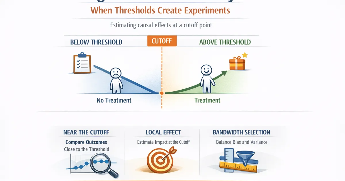
How regression discontinuity designs exploit score cutoffs to estimate causal effects. A practical guide for product analysts with real-world examples.
Quick Hits
- •RDD exploits situations where treatment is assigned based on whether a continuous score crosses a cutoff, creating a natural experiment near the threshold
- •Users just above and just below the cutoff are nearly identical on all characteristics, so comparing their outcomes isolates the treatment effect
- •RDD estimates a local effect at the cutoff, not a global treatment effect for the entire population
- •Bandwidth selection controls the bias-variance tradeoff: too narrow loses precision, too wide introduces bias from observations far from the cutoff
- •Manipulation of the running variable (users gaming the threshold) is the primary threat to RDD validity and must always be tested
TL;DR
Regression discontinuity designs (RDD) let you estimate causal effects whenever treatment is assigned based on whether a continuous score crosses a threshold. By comparing observations just above and just below the cutoff, you create a quasi-experiment where units are nearly identical in everything except treatment status. RDD is one of the most internally valid observational designs, but it only tells you about the effect at the threshold, and it breaks down if users can manipulate their score.
The Key Insight
Many product decisions involve thresholds. Users with a risk score above 70 get flagged for review. Accounts with more than 1,000 monthly active users qualify for enterprise pricing. Sellers with ratings below 4.0 lose their featured placement.
These thresholds create a natural experiment. A user with a score of 71 received treatment (the flag, the pricing tier, the delisting), while a user with a score of 69 did not. But these two users are nearly identical in every other way -- their scores differ by a tiny amount, and all the characteristics that determine their score are virtually the same.
By comparing outcomes for observations in a narrow window around the cutoff, you effectively have a randomized experiment at the threshold. The key assumption is that there is no other discontinuity at the cutoff that could confound the comparison.
Sharp vs. Fuzzy RDD
Sharp RDD
In a sharp design, treatment is a deterministic function of the running variable:
Everyone above the cutoff is treated. Everyone below is untreated. The causal effect is the discontinuity in the outcome at the cutoff:
Fuzzy RDD
In a fuzzy design, crossing the cutoff increases the probability of treatment but does not guarantee it. Some users above the cutoff are untreated (perhaps they opt out), and some below are treated (perhaps through an exception process).
Fuzzy RDD is structurally identical to an instrumental variables problem: the cutoff indicator is an instrument for treatment status. The estimate is a LATE for compliers at the threshold.
Implementation: Step by Step
1. Identify the Running Variable and Cutoff
The running variable must be continuous (or at least take many distinct values), and the cutoff must be well-defined. Document the exact rule that determines treatment assignment. If the assignment rule is ambiguous or changed over time, RDD may not be appropriate.
2. Visualize the Data
Plot the outcome variable against the running variable. If there is a causal effect, you should see a visible jump at the cutoff. This is the most important diagnostic. If the jump is invisible in the raw scatter plot, a statistically significant RDD estimate should be viewed skeptically.
Also plot the density of the running variable near the cutoff (the McCrary test). A discontinuity in the density suggests manipulation -- users sorting themselves to one side of the threshold.
3. Choose the Estimation Method
The standard approach is local polynomial regression: fit separate polynomial functions of the running variable on each side of the cutoff, within a specified bandwidth. The causal effect is the difference in predicted values at the cutoff.
- Linear local regression (order 1) is the default and usually preferred near the boundary.
- Quadratic or higher-order polynomials can accommodate curvature but may overfit.
- Global high-order polynomials (fitting a 5th-degree polynomial to all data) are strongly discouraged. They are sensitive to outliers and produce unreliable estimates.
4. Select the Bandwidth
The bandwidth determines how much data near the cutoff you use. Narrower bandwidths reduce bias (observations farther from the cutoff are less comparable) but increase variance (fewer observations means less precision).
Use data-driven selectors:
- Imbens-Kalyanaraman (IK): The classic optimal bandwidth selector.
- Calonico-Cattaneo-Titiunik (CCT): An improved selector with better finite-sample properties and honest confidence intervals.
Always report results for the optimal bandwidth, half the optimal bandwidth, and double the optimal bandwidth. If results are sensitive to bandwidth choice, the estimate is fragile.
5. Estimate the Treatment Effect
Using the rdrobust package (available in R and Python), estimate the local treatment effect at the cutoff with bias-corrected confidence intervals.
A Product Analytics Example
Your platform assigns users an "engagement score" from 0 to 100 based on login frequency, feature usage, and content creation. Users scoring 75 or above receive a personalized recommendation feed. You want to know if the recommendation feed increases purchases.
Running variable: Engagement score (continuous, 0-100). Cutoff: 75. Treatment: Personalized recommendations. Outcome: Purchases in the next 30 days.
Steps:
- Plot purchases against engagement score. Look for a jump at 75.
- Run the McCrary density test. If users are gaming their engagement score to reach 75, you will see bunching just above the cutoff.
- Estimate the effect using local linear regression with the CCT bandwidth selector.
- Check covariate balance at the cutoff: account age, device type, subscription tier should be smooth through the threshold.
- Report the LATE at the cutoff with bias-corrected CIs and sensitivity across bandwidths.
Result interpretation: The estimated 12% increase in purchases applies specifically to users near the 75-point threshold. It does not tell you what would happen if you gave recommendations to all users or moved the threshold to 50.
Validity Checks
No Manipulation (McCrary Test)
If users can precisely control their score to land above the threshold, the comparison breaks down. The McCrary density test checks for a jump in the running variable's density at the cutoff. A significant jump is a red flag.
In product contexts: Ask whether users can see their score and whether they have incentives and ability to game it. A credit score threshold is easier to manipulate than an internal algorithm score users never see.
Covariate Smoothness
Pre-treatment covariates should be continuous through the cutoff. If account age, device type, or geographic distribution shows a discontinuity at the threshold, something other than the treatment is changing at the cutoff.
Placebo Cutoffs
Estimate the "effect" at fake cutoffs (values away from the real threshold). If you detect significant jumps at arbitrary points, your design has problems -- either the outcome is noisy, the functional form is wrong, or there are other discontinuities in the data.
Sensitivity to Bandwidth
Results should be qualitatively stable across reasonable bandwidth choices. If the sign or significance of the effect changes dramatically between the optimal bandwidth and half the optimal bandwidth, the estimate is not credible.
Limitations
Local effect only. RDD estimates the treatment effect at the cutoff. It does not tell you about the effect for users far from the threshold. Extrapolation is risky.
Requires a continuous running variable. With a discrete running variable (like "number of logins"), the quasi-random comparison argument weakens because observations at adjacent values may not be comparable.
Low power. Because RDD only uses data near the cutoff, it can be underpowered. You need a substantial amount of data clustered around the threshold.
Functional form sensitivity. The choice of polynomial order and bandwidth affects the estimate. While data-driven methods help, some researcher judgment is unavoidable.
When to Reach for RDD
RDD is the right tool when:
- Treatment is assigned by a score cutoff (even if the rule is not perfectly enforced -- that is the fuzzy case).
- The running variable is continuous or has many distinct values.
- Users cannot precisely manipulate their position relative to the cutoff.
- You have enough observations near the threshold for adequate power.
If these conditions hold, RDD is among the most credible quasi-experimental designs available. For situations that don't fit the RDD framework, consider difference-in-differences, instrumental variables, or propensity score matching. For an overview of all approaches, see our causal inference pillar post.
References
- https://www.journals.uchicago.edu/doi/10.1086/675536
- https://rdpackages.github.io/
- https://cattaneo.princeton.edu/books/Cattaneo-Idrobo-Titiunik_2020_CUP.pdf
Frequently Asked Questions
What is the difference between sharp and fuzzy RDD?
How do I choose the bandwidth for RDD?
Can I use RDD when the running variable is discrete?
Key Takeaway
Regression discontinuity is one of the most credible quasi-experimental designs because it exploits a sharp rule-based assignment, but it only estimates a local effect at the threshold and requires that users cannot manipulate their score to cross the cutoff.