Contents
Propensity Score Matching: Balancing Groups Without Randomization
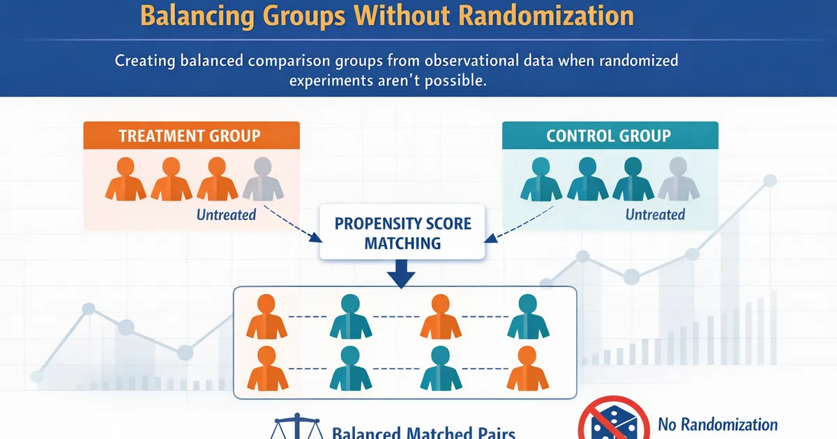
Learn how propensity score matching creates balanced comparison groups from observational data when randomized experiments aren't possible.
Quick Hits
- •Propensity score matching reduces the dimensionality problem: instead of matching on dozens of covariates individually, you match on a single summary score
- •The propensity score is the probability of receiving treatment given observed covariates -- estimated via logistic regression, gradient boosting, or other classifiers
- •Matching quality is assessed by covariate balance, not by model fit metrics like AUC or accuracy
- •PSM only handles observed confounders; unmeasured confounding remains a threat, and sensitivity analysis is essential
- •Common pitfalls include matching on post-treatment variables, discarding too many unmatched units, and ignoring the matched-sample design in downstream analysis
TL;DR
Propensity score matching lets you create an approximate experiment from observational data by pairing treated and untreated observations that had similar probabilities of receiving treatment. When done well, it balances measured confounders and isolates the treatment effect. When done poorly -- or when unmeasured confounders lurk -- it gives you false confidence in a biased estimate. This post covers the mechanics, practical implementation, diagnostics, and limitations every analyst should know.
The Problem PSM Solves
In a randomized experiment, treatment and control groups are comparable by construction. In observational data, they are not. Users who adopt a new feature differ from those who don't in ways that also affect the outcome you care about.
Suppose you want to measure the effect of adopting a premium subscription on 12-month retention. Premium users are more engaged, have been on the platform longer, and use more features. Comparing their retention to free-tier users directly conflates the subscription effect with all those pre-existing differences.
You need to compare premium users to free-tier users who look like they could have subscribed but didn't. That is what propensity score matching does.
How Propensity Score Matching Works
Step 1: Estimate the Propensity Score
The propensity score is the probability that a user receives treatment given their observed covariates:
You estimate this with a classification model -- most commonly logistic regression, though gradient boosted trees and random forests are increasingly used. The model predicts treatment assignment (not the outcome) using pre-treatment covariates.
Critical rule: Only include pre-treatment variables. Including post-treatment variables (things that happened after or because of treatment) introduces post-treatment bias and invalidates the analysis.
Step 2: Match Treated to Untreated Units
Once every observation has a propensity score, you pair each treated unit with one or more untreated units that have similar scores. Common approaches:
- Nearest-neighbor matching: Each treated unit is matched to the untreated unit with the closest propensity score.
- Caliper matching: Same as nearest-neighbor, but matches are only accepted if the score difference is within a specified threshold (caliper). A common caliper is 0.2 standard deviations of the logit of the propensity score.
- Full matching: Creates optimally balanced strata containing at least one treated and one untreated unit.
- Mahalanobis distance within propensity score calipers: Matches on both the propensity score and key covariates directly.
Matching can be done with or without replacement. Matching with replacement improves match quality (each untreated unit can serve as a match for multiple treated units) but complicates variance estimation.
Step 3: Assess Balance
This is the most important diagnostic step. After matching, check whether the distribution of each covariate is similar across treated and matched control groups. Use:
- Standardized mean differences (SMD): Values below 0.1 indicate good balance. This is the primary metric.
- Variance ratios: Should be close to 1.
- Visual inspection: Plot covariate distributions before and after matching.
If balance is poor, iterate: try different matching algorithms, add interaction terms or nonlinear terms to the propensity score model, or use a different estimation approach entirely.
A common misconception: People evaluate the propensity score model using AUC, accuracy, or other prediction metrics. This is wrong. The goal is covariate balance in the matched sample, not prediction accuracy. A model with mediocre AUC can produce excellent balance, and vice versa.
Step 4: Estimate the Treatment Effect
On the matched sample, estimate the average treatment effect on the treated (ATT) by comparing outcomes:
where is the matched control for treated unit .
For more robust estimates, run a regression on the matched sample (doubly robust estimation). This protects against either the propensity score model or the outcome model being slightly misspecified.
A Practical Example: Measuring Onboarding Impact
Your company redesigned its onboarding flow. Unfortunately, the rollout was not randomized -- it went to new users who signed up through a specific marketing channel. You want to know if the new onboarding increased 30-day activation.
Covariates for the propensity model: Sign-up source (organic, paid, referral), device type, country, day of week, referral status, and any pre-activation engagement signals captured during sign-up.
Process:
- Fit a logistic regression predicting new-onboarding assignment from these covariates.
- Apply nearest-neighbor matching with a caliper of 0.2 SD on the logit propensity score.
- Check SMDs: if sign-up source, device type, and country all have SMDs below 0.1 after matching, balance is acceptable.
- Compare 30-day activation rates between matched groups.
- Run a sensitivity analysis to assess how strong an unmeasured confounder (e.g., user intent or motivation) would need to be to explain away the result.
Limitations and Common Pitfalls
The Unmeasured Confounding Problem
PSM only adjusts for observed covariates. If an unmeasured variable drives both treatment selection and the outcome, the estimate is biased. This is the single biggest limitation. You cannot test for unmeasured confounders directly, but you can:
- Use Rosenbaum bounds to quantify sensitivity to hidden bias.
- Compute the E-value to determine how strong a confounder would need to be.
- Argue substantively (using domain knowledge) that the key confounders are measured.
Overlap Violations
If treated and untreated groups have very different propensity score distributions, many treated units have no good match. This is a structural problem, not a statistical one. If the groups barely overlap, no matching method can save you. Check the region of common support and consider trimming extreme propensity scores.
Matching on Post-Treatment Variables
Including variables affected by the treatment in the propensity model is one of the most common and most damaging mistakes. If adopting the premium tier causes users to use more features, including feature usage in the model blocks part of the causal pathway and biases the estimate.
Ignoring the Matched Design
After matching, the data has a paired structure. Standard errors should account for this via cluster-robust standard errors, bootstrap methods, or matched-pair analysis. Treating the matched sample as if it were a simple random sample understates uncertainty.
PSM vs. Alternatives
| Method | Strengths | Weaknesses |
|---|---|---|
| PSM | Transparent balance checking, intuitive | Discards unmatched units, only handles observed confounders |
| Inverse Probability Weighting (IPW) | Uses all data, no discarding | Sensitive to extreme weights |
| Doubly Robust (DR) | Robust if either outcome or PS model is correct | More complex to implement |
| Coarsened Exact Matching (CEM) | Exact balance on coarsened covariates | Curse of dimensionality with many covariates |
In practice, doubly robust estimation -- combining a propensity score model with an outcome regression -- is the modern best practice. It gives you a consistent estimate if either model is correct, and improved efficiency when both are reasonable.
When to Use PSM in Product Analytics
Propensity score matching is a good fit when:
- You have a clear treatment/control comparison with no randomization.
- You have rich pre-treatment covariate data in your event logs and user tables.
- The overlap between treated and untreated groups is reasonable.
- You can make a credible case that the important confounders are measured.
It is a poor fit when:
- Treatment assignment is driven primarily by unobserved factors (motivation, intent).
- There is little covariate overlap between groups.
- You have access to structural features (thresholds, instruments, time variation) that would support stronger methods like regression discontinuity or instrumental variables.
For a broader view of when to use PSM versus other causal methods, see our causal inference overview.
References
- https://academic.oup.com/biomet/article-abstract/70/1/41/240879
- https://www.jstatsoft.org/article/view/v042i08
- https://gking.harvard.edu/publications/why-propensity-scores-should-not-be-used-formatching
Frequently Asked Questions
What is the difference between propensity score matching and regression adjustment?
How do I choose between nearest-neighbor, caliper, and full matching?
Can I use propensity score matching with small sample sizes?
Key Takeaway
Propensity score matching approximates a randomized experiment by creating balanced comparison groups from observational data, but its validity depends entirely on the assumption that you have measured all relevant confounders.