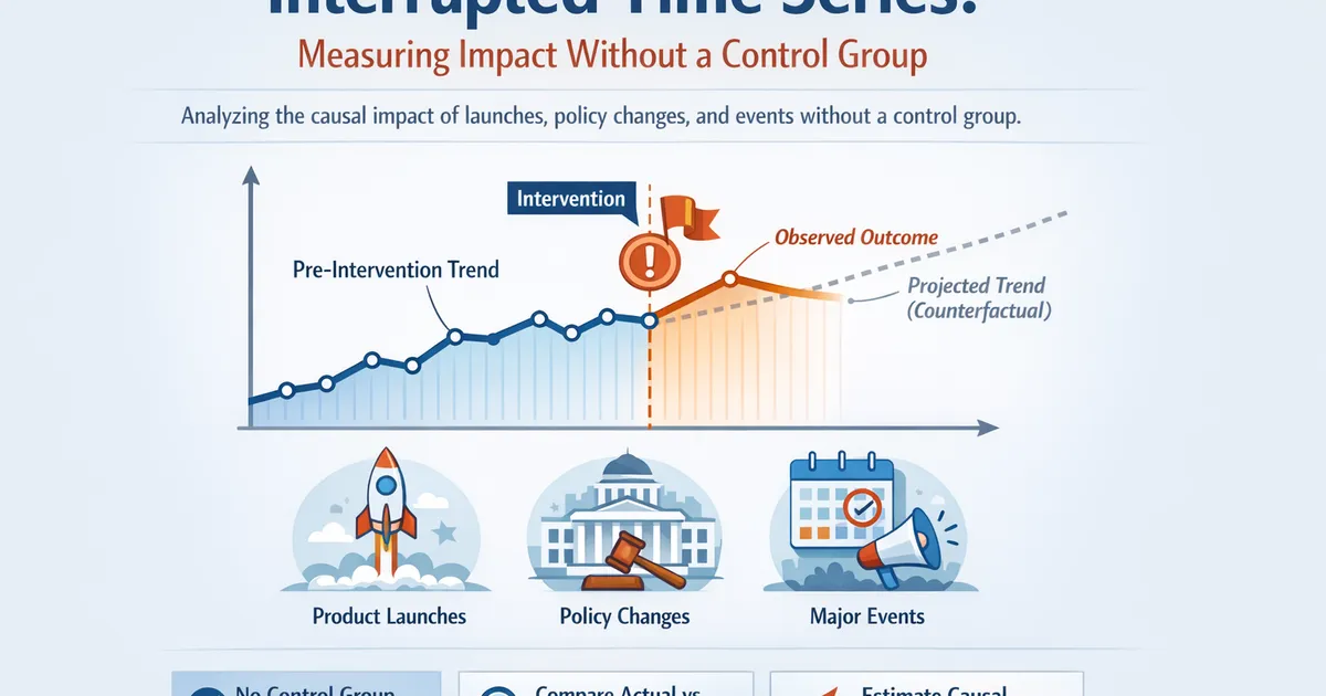
Interrupted Time Series: Measuring Impact Without a Control Group

TL;DR

You launched a feature, changed a policy, or rolled out an algorithm update to all users. There is no control group. How do you measure impact? Interrupted time series (ITS) analysis compares the post-intervention metric trajectory to the projected pre-intervention trend. If the metric deviates significantly from where it was heading, you have evidence of a causal effect. This guide covers the method, assumptions, implementation, and pitfalls.

When You Need ITS

Not every product change can be A/B tested. Some situations demand ITS:

• Site-wide changes: New pricing, redesigned checkout flow, updated algorithm affecting all users
• Policy or regulatory changes: GDPR implementation, new content moderation policy
• External events: Competitor launches, market shifts, viral moments
• Infrastructure changes: Backend migration, CDN change, performance optimization
• Retrospective analysis: A change was made without an experiment, and leadership wants to know the impact

In all these cases, the intervention affects everyone at once. There is no randomized control group. ITS provides causal inference under weaker assumptions than a randomized experiment but stronger assumptions than simple pre/post comparison.

How ITS Works

The Core Idea

ITS fits a regression model to the pre-intervention data to establish the baseline trajectory (trend and level). It then projects this model into the post-intervention period to create a counterfactual -- what would have happened without the intervention. The difference between the actual post-intervention data and the counterfactual is the estimated effect.

The Segmented Regression Model

The standard ITS model is:

$Y_t = \beta_0 + \beta_1 T + \beta_2 D + \beta_3 P + \epsilon_t$

Where:

• $Y_t$ is the outcome at time $t$
• $T$ is the time variable (1, 2, 3, ...)
• $D$ is a dummy variable (0 before intervention, 1 after)
• $P$ is the time since intervention (0 before, 1, 2, 3, ... after)

Interpreting the coefficients:

• $\beta_0$: Baseline level at time zero
• $\beta_1$: Pre-intervention slope (trend before the change)
• $\beta_2$: Immediate level change at the intervention point
• $\beta_3$: Change in slope after the intervention

This is powerful because it separates two types of effects: an immediate jump (or drop) and a change in trajectory.

Example: Onboarding Redesign

You redesigned your onboarding flow on day 60. DAU was trending up at roughly 20 users per day before the redesign.

import numpy as np
import pandas as pd
import statsmodels.api as sm

# Create ITS variables
n = 120  # 60 days pre, 60 days post
df = pd.DataFrame({
    'time': range(1, n + 1),
    'intervention': [0]*60 + [1]*60,
    'time_after': [0]*60 + list(range(1, 61)),
    'dau': daily_dau_values
})

# Fit ITS model with Newey-West standard errors
X = sm.add_constant(df[['time', 'intervention', 'time_after']])
model = sm.OLS(df['dau'], X).fit(cov_type='HAC',
                                   cov_kwds={'maxlags': 7})
print(model.summary())

If $\beta_2 = 500$ (p < 0.01) and $\beta_3 = 10$ (p = 0.03), you can conclude: "The onboarding redesign produced an immediate increase of 500 DAU and accelerated the growth rate by 10 additional users per day."

The Critical Assumption: No Confounders at the Break Point

ITS assumes that without the intervention, the pre-intervention trend would have continued. This is the continuity assumption (sometimes called the "no history threat" assumption).

This assumption is violated when:

• Another change happened simultaneously (a marketing campaign launched the same day)
• An external event coincided (a competitor shut down, a holiday occurred)
• The intervention was triggered by an unusual event (you redesigned after a crash -- the crash itself caused the dip, and regression to the mean causes the recovery)

How to strengthen the assumption:

1. Control series: Include a metric that should NOT be affected by the intervention. If it also shows a shift, something external happened.
2. Multiple baselines: Apply ITS to different subgroups or markets. If only the affected group shows a change, the evidence is stronger.
3. Documentation: Record all known concurrent changes to argue that the intervention is the most plausible cause.
4. Placebo tests: Run the same analysis at fake intervention points (before the real one). If you find "effects" at random points, your method is unreliable.

Google's CausalImpact: Bayesian ITS

Google's CausalImpact package implements a Bayesian approach to ITS. Instead of segmented regression, it builds a structural time series model from the pre-intervention data and uses it to generate a posterior predictive distribution for the counterfactual.

# Using the Python port of CausalImpact
from causalimpact import CausalImpact

data = pd.DataFrame({
    'y': daily_metric,
    'x1': control_metric  # optional control series
}, index=dates)

pre_period = ['2025-01-01', '2025-03-01']
post_period = ['2025-03-02', '2025-04-30']

ci = CausalImpact(data, pre_period, post_period)
print(ci.summary())
ci.plot()

Advantages of CausalImpact:

• Provides credible intervals for the cumulative and pointwise effect
• Can incorporate control series (covariates) to improve the counterfactual
• Handles seasonality through the underlying state space model
• Returns a probability that the effect is real

When to use CausalImpact vs. segmented regression:

• CausalImpact: When you have control series, want probabilistic statements, or need to handle complex seasonality
• Segmented regression: When you want simplicity, transparent coefficient interpretation, or need to test for slope changes explicitly

Handling Seasonality and Autocorrelation in ITS

Seasonality

If your metric has weekly or seasonal patterns, failing to account for them will bias your ITS estimates. Two approaches:

1. Include seasonal terms in the regression: Add day-of-week dummy variables or Fourier terms to the ITS model.
2. Deseasonalize first: Apply STL decomposition and run ITS on the deseasonalized (trend + residual) series.

Autocorrelation

ITS on daily data will almost certainly have autocorrelated residuals. Use Newey-West standard errors (as shown in the example above) or fit an ARIMA-based ITS model that explicitly models the autocorrelation.

# ITS with seasonal terms and HAC standard errors
df['dow'] = df.index.dayofweek  # 0=Monday, 6=Sunday
dow_dummies = pd.get_dummies(df['dow'], prefix='dow', drop_first=True)

X = pd.concat([
    sm.add_constant(df[['time', 'intervention', 'time_after']]),
    dow_dummies
], axis=1)

model = sm.OLS(df['dau'], X).fit(cov_type='HAC',
                                   cov_kwds={'maxlags': 7})

Design Considerations

How Much Pre-Intervention Data?

More is generally better, but very old data may reflect a different product reality. Rules of thumb:

• Minimum: 8-10 data points (strict minimum for segmented regression)
• Comfortable: 30-60 data points (for daily data, 1-2 months)
• Ideal: Enough to capture at least 2 full seasonal cycles

How Long After the Intervention?

Long enough to distinguish a sustained effect from a novelty effect or temporary disruption. For product changes:

• Minimum: 2-4 weeks (to capture at least one full weekly cycle post-intervention)
• Watch for: Effects that fade over time (novelty wearing off) or effects that grow (adoption curves)

Pre-Registration

Like A/B tests, pre-register your ITS analysis. Specify the intervention date, the outcome metric, the model specification, and what constitutes a meaningful effect size BEFORE looking at the post-intervention data.

Limitations

ITS is powerful but not omnipotent:

• Cannot isolate confounders: Without a control group, you can never be 100% certain the intervention (and nothing else) caused the change.
• Assumes stable pre-trend: If the pre-intervention period was itself unusual, the counterfactual projection will be wrong.
• Requires enough data: Short time series produce unstable estimates.
• Sensitive to model specification: Different model choices (linear vs. nonlinear trend, inclusion of seasonality) can change results. Report sensitivity analyses.

For situations where you have a comparison group, difference-in-differences strengthens the causal claim by combining pre/post comparison with a control group.

References

- https://doi.org/10.1016/j.jclinepi.2016.12.001
- https://google.github.io/CausalImpact/CausalImpact.html
- https://ds4ps.org/pe4ps-textbook/docs/p-020-time-series.html
- Bernal, J. L., Cummins, S., & Gasparrini, A. (2017). Interrupted time series regression for the evaluation of public health interventions. *International Journal of Epidemiology*, 46(1), 348-355.
- Brodersen, K. H., Gallusser, F., Koehler, J., Remy, N., & Scott, S. L. (2015). Inferring causal impact using Bayesian structural time-series models. *Annals of Applied Statistics*, 9(1), 247-274.
Frequently Asked Questions
When should I use ITS instead of a standard A/B test?
How many time points do I need before and after the intervention?
What if something else changed at the same time as my intervention?
Key Takeaway
Interrupted time series is the go-to method for measuring the causal impact of a change when you have no control group. It projects the pre-intervention trend into the post period as a counterfactual and measures the deviation. The key assumption -- that the pre-trend would have continued -- must be carefully defended.