Contents
Instrumental Variables: Finding Natural Experiments in Product Data
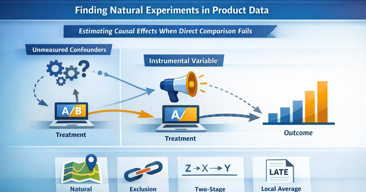
How instrumental variables let you estimate causal effects when unmeasured confounding makes direct comparison impossible. Practical IV examples for tech.
Quick Hits
- •An instrumental variable is a source of quasi-random variation in treatment that only affects the outcome through the treatment itself
- •IV estimates are consistent even with unmeasured confounders, unlike propensity score matching or regression adjustment
- •The exclusion restriction -- that the instrument affects the outcome only via treatment -- is the critical assumption and cannot be tested statistically
- •Weak instruments (low first-stage F-statistic) cause severe bias and inflated standard errors; always check the first stage
- •IV estimates a Local Average Treatment Effect (LATE) for compliers, not the Average Treatment Effect for everyone
TL;DR
Instrumental variables let you estimate causal effects even when you cannot measure or adjust for all confounders. The trick is finding a variable (the instrument) that nudges treatment quasi-randomly without affecting the outcome through any other channel. When you find a good instrument, you get a consistent causal estimate. When you don't, you get a biased mess that looks precise. This post covers how IV works, where to find instruments in product data, how to implement two-stage least squares, and the diagnostics that separate credible IV studies from wishful thinking.
When You Need an Instrument
Most causal inference methods for observational data assume you can measure all confounders. Propensity score matching requires conditional ignorability. Regression adjustment requires correct functional form and no omitted variables.
But what if unmeasured confounding is unavoidable? User motivation, technical sophistication, and intent are hard to measure directly. If these unmeasured factors drive both treatment adoption and the outcome, conditioning on observed covariates is not enough.
Instrumental variables solve this by finding variation in treatment that is unrelated to confounders. Instead of trying to adjust for everything, you isolate the portion of treatment variation that is "as good as random."
The Three IV Assumptions
An instrumental variable must satisfy:
1. Relevance
The instrument must predict treatment. must have a non-trivial effect on the probability or intensity of treatment . This is testable: estimate the first-stage regression and check the F-statistic on the instrument. A rule of thumb is F > 10 for a single instrument (and the more modern Stock-Yogo critical values for weak instrument detection).
2. Independence (Exogeneity)
The instrument must be unrelated to unmeasured confounders. must be "as good as random" with respect to factors that affect the outcome. This is partially testable: you can check whether the instrument is balanced on observed covariates. But balance on observables does not guarantee balance on unobservables, so this assumption ultimately requires a substantive argument.
3. Exclusion Restriction
The instrument must affect the outcome only through the treatment. There should be no direct effect of on other than through . This is the hardest assumption and is not statistically testable. It must be argued from domain knowledge.
If any of these three fails, the IV estimate is biased and potentially worse than a naive comparison.
Two-Stage Least Squares (2SLS)
The standard IV estimator is two-stage least squares:
First stage: Regress treatment on the instrument (and any control variables ):
Second stage: Regress the outcome on the predicted treatment from the first stage (and controls):
The coefficient is the IV estimate of the causal effect. It uses only the variation in treatment that is driven by the instrument, effectively purging confounded variation.
Finding Instruments in Product Data
Good instruments are rare, but tech companies have structural features that create them.
Randomized Encouragements
If you ran an A/B test that encouraged users to adopt a feature (without forcing them), the random assignment to encouragement is an instrument for actual adoption. This is the encouragement design, and it is one of the cleanest instrument sources.
Example: You randomly assigned half of users to receive a tooltip promoting your advanced analytics dashboard. The tooltip increased dashboard adoption by 15 percentage points. Using tooltip assignment as an instrument for dashboard usage, you estimate the causal effect of the dashboard on user retention.
Server-Side or Infrastructure Variation
Latency differences caused by server assignment, CDN routing, or load balancing create exogenous variation in user experience. If users assigned to a faster server (due to random load balancing) experience lower latency, server assignment is an instrument for page load speed.
Example: You want to know how page load time affects purchases. Users are quasi-randomly assigned to servers with different response times. Server assignment predicts load time (relevant) and plausibly does not affect purchases through any other channel (exclusion restriction).
Geographic or Temporal Rollouts
Features rolled out in stages across regions or time periods create variation that may be unrelated to user characteristics. If the rollout order was determined by engineering convenience (not by market potential), geography or rollout wave is a candidate instrument.
Example: A payments feature launched in Germany before France due to regulatory timing. If the timing was driven by regulatory approval (exogenous) rather than business priorities (endogenous), country-wave is an instrument for feature access.
Network Exposure
In social products, the fraction of a user's friends who were treated can serve as an instrument. If friends' treatment was randomized, the share of treated friends is quasi-random from the focal user's perspective and predicts the focal user's likelihood of adoption.
Diagnostics and Red Flags
Weak Instruments
If the first-stage F-statistic is below 10, the instrument barely predicts treatment. Weak instruments cause:
- Severe finite-sample bias (IV estimates are biased toward OLS).
- Wildly inflated standard errors.
- Unreliable confidence intervals.
Fix: Find a stronger instrument, combine multiple weak instruments (carefully), or use weak-instrument robust inference methods (Anderson-Rubin confidence sets).
Over-Identification Tests
If you have more instruments than endogenous variables, you can test the over-identifying restrictions. The Sargan-Hansen J-test checks whether the instruments give consistent estimates. Rejection suggests at least one instrument violates the exclusion restriction. But passing does not guarantee all instruments are valid -- it only means they agree with each other.
Exclusion Restriction Violations
This is the make-or-break assumption. Ask yourself: is there any plausible channel through which the instrument affects the outcome other than through treatment?
For the push-notification instrument above: could the notification itself (independent of dashboard usage) affect retention? If the notification reminds users the product exists, and that reminder itself boosts retention, the exclusion restriction is violated.
Think hard. Challenge your assumption. Have colleagues try to poke holes. This is where IV analyses live or die.
What IV Actually Estimates: LATE
A subtle but important point: with a binary instrument and binary treatment, IV estimates the Local Average Treatment Effect (LATE) -- the effect for compliers. Compliers are units whose treatment status is changed by the instrument.
There are four types:
- Compliers: Treated when , untreated when . IV estimates the effect for these users.
- Always-takers: Treated regardless of .
- Never-takers: Untreated regardless of .
- Defiers: Treated when , untreated when . (Assumed to not exist under monotonicity.)
If you want to generalize beyond compliers, you need additional assumptions or a different method.
IV in Practice: A Step-by-Step Guide
- Identify a candidate instrument. Look for exogenous variation in treatment: randomized encouragements, infrastructure quirks, rollout timing.
- Argue the exclusion restriction. Write down every possible channel from to . If any bypass , the instrument is invalid.
- Test relevance. Run the first-stage regression. Check the F-statistic. If below 10, stop.
- Check instrument exogeneity. Examine whether the instrument is balanced on observed covariates. Run placebo tests on pre-treatment outcomes.
- Estimate the second stage. Use 2SLS with proper standard errors (heteroskedasticity-robust or clustered).
- Report LATE, not ATE. Be explicit about who your estimate applies to.
- Run sensitivity analysis. How much would a violation of the exclusion restriction need to change the reduced-form relationship to nullify the result?
For broader context on when IV is the right choice versus other methods, see our causal inference overview.
Common Mistakes
- Using outcome-related variables as instruments. If the variable predicts the outcome directly, the exclusion restriction fails.
- Ignoring weak instruments. An F-statistic of 3 does not become acceptable just because you want it to.
- Claiming ATE when you have LATE. Be honest about the population your estimate covers.
- Cherry-picking instruments. Trying multiple instruments and reporting only the one that gives the desired result invalidates inference.
- Forgetting controls. If the instrument is conditionally exogenous (valid only after conditioning on covariates), those covariates must be included in both stages.
Instrumental variables are among the most powerful tools in the causal inference toolkit, but they are also the most demanding. A credible IV analysis requires a genuine source of exogenous variation and an honest, substantive defense of the exclusion restriction.
References
- https://www.jstor.org/stable/2951620
- https://www.nber.org/papers/w0172
- https://mixtape.scunning.com/06-regression_discontinuity
Frequently Asked Questions
What makes a good instrumental variable?
Why are IV estimates often imprecise?
What is the difference between LATE and ATE?
Key Takeaway
Instrumental variables let you sidestep unmeasured confounding by exploiting quasi-random variation in treatment, but their validity depends on the exclusion restriction, which must be argued from domain knowledge rather than tested statistically.