Contents
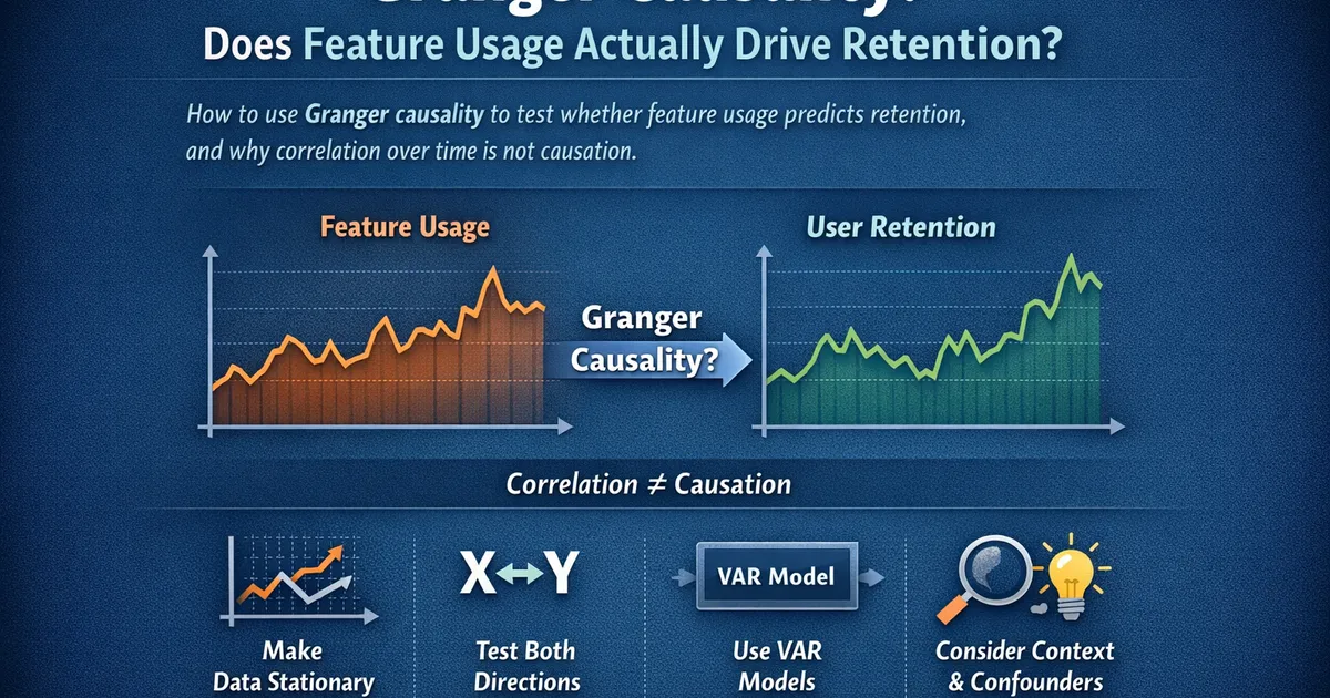
Granger Causality: Does Feature Usage Actually Drive Retention?
How to use Granger causality to test whether feature usage predicts retention, and why correlation over time is not causation.
Quick Hits
- •Granger causality tests whether X predicts Y beyond Y's own history -- not true causation
- •Two metrics can be correlated over time simply because both have trends -- always difference first
- •The test requires stationary time series -- apply differencing or detrending before running it
- •Reverse causality is common: retention might drive feature usage, not the other way around
- •Use VAR models to test bidirectional Granger causality simultaneously
TL;DR
Your product team believes that feature usage drives retention. But does past feature usage actually predict future retention, or are both just trending up together? Granger causality provides a statistical framework for testing this. It asks: do past values of feature usage improve predictions of retention beyond what retention's own past values provide? This guide covers the method, implementation, interpretation, and the crucial caveats about what Granger causality does and does not prove.
The Question Every Product Team Asks
"Users who use Feature X have higher retention." This observation is ubiquitous in product analytics. But it raises a critical question: does Feature X drive retention, or do retained users simply use more features?
Correlation between two metrics at the same point in time cannot answer this. Even looking at the time series -- feature usage going up while retention goes up -- does not help, because both might be responding to a third factor (a marketing push, a seasonal cycle, organic growth).
Granger causality offers a structured approach: does knowing the past of feature usage help predict the future of retention, even after accounting for retention's own past? If yes, there is a temporal predictive relationship that is at least consistent with (though not proof of) a causal mechanism.
What Granger Causality Means
The Formal Definition
Granger-causes if past values of contain information that helps predict beyond what past values of alone provide.
Formally, Granger-causes if:
In other words, the forecast error for is smaller when you include past than when you use past alone.
What It Is
- A test for temporal precedence: Does lead in time?
- A test for incremental predictive power: Does add information beyond 's own history?
- A structured way to assess lead-lag relationships between product metrics
What It Is Not
- Not proof of causation: A third variable might drive both and with different lags
- Not a mechanism: It does not tell you how affects
- Not immune to confounding: Unmeasured variables can create spurious Granger causality
Prerequisites: Making Data Stationary
Why Stationarity Matters
Granger causality tests assume stationary time series. Non-stationary data (data with trends, unit roots, or changing variance) produces spurious results. Two unrelated metrics that both trend upward will appear to Granger-cause each other.
Testing for Stationarity
Use the Augmented Dickey-Fuller (ADF) test:
from statsmodels.tsa.stattools import adfuller

# Test feature_usage for stationarity
result = adfuller(feature_usage, maxlag=14, regression='ct')
print(f"ADF Statistic: {result[0]:.4f}")
print(f"p-value: {result[1]:.4f}")
# p > 0.05 => non-stationary, needs differencing
Achieving Stationarity
If either series is non-stationary (p > 0.05 on the ADF test), apply differencing:
# First differencing: compute day-over-day changes
feature_usage_diff = feature_usage.diff().dropna()
retention_diff = retention.diff().dropna()
Re-test with ADF after differencing. Most product metrics become stationary after first differencing. If not, apply second differencing.
Important: After differencing, you are testing whether changes in feature usage predict changes in retention, rather than whether levels predict levels. This is actually the more meaningful question for most product contexts.
Running the Granger Causality Test
Implementation
from statsmodels.tsa.stattools import grangercausalitytests
import pandas as pd

# Combine into a DataFrame (Y first, X second)
data = pd.DataFrame({
    'retention': retention_diff,
    'feature_usage': feature_usage_diff
}).dropna()

# Test: Does feature_usage Granger-cause retention?
print("Does feature usage Granger-cause retention?")
result = grangercausalitytests(
    data[['retention', 'feature_usage']],
    maxlag=14
)
The function tests at each lag from 1 to maxlag and reports four test statistics. The F-test is the standard one to report.
Interpreting Results
The output shows p-values for each lag:
Lag 1: F-test p-value = 0.0023  (significant)
Lag 2: F-test p-value = 0.0041  (significant)
...
Lag 7: F-test p-value = 0.0156  (significant)
Lag 8: F-test p-value = 0.1234  (not significant)
This would suggest that feature usage from 1-7 days ago helps predict today's retention. The lag structure is itself informative: a 1-7 day lag aligns with the idea that weekly feature usage affects weekly retention.
Testing Both Directions
Always test bidirectional causality:
# Does retention Granger-cause feature_usage?
print("Does retention Granger-cause feature usage?")
result_reverse = grangercausalitytests(
    data[['feature_usage', 'retention']],
    maxlag=14
)
Four possible outcomes:
| Feature -> Retention | Retention -> Feature | Interpretation |
|---|---|---|
| Significant | Not significant | Feature usage predicts retention (consistent with feature driving retention) |
| Not significant | Significant | Retention predicts feature usage (retained users use features more) |
| Significant | Significant | Feedback loop (both predict each other) |
| Not significant | Not significant | No temporal predictive relationship |
VAR Models: The Multivariate Framework
Beyond Pairwise Tests
Granger causality between two variables can be confounded by a third. Vector Autoregression (VAR) models extend the framework to multiple variables simultaneously.
from statsmodels.tsa.api import VAR

# Include multiple metrics
data = pd.DataFrame({
    'retention': retention_diff,
    'feature_usage': feature_usage_diff,
    'sessions': sessions_diff,
    'support_tickets': support_diff
}).dropna()

# Fit VAR model
model = VAR(data)
lag_order = model.select_order(maxlags=14)
print(lag_order.summary())  # Select optimal lag via AIC/BIC

results = model.fit(lag_order.aic)
print(results.summary())
Granger Causality in VAR
After fitting the VAR, test Granger causality while controlling for other variables:
# Test: Does feature_usage Granger-cause retention,
# controlling for sessions and support_tickets?
gc_result = results.test_causality(
    'retention',
    ['feature_usage'],
    kind='f'
)
print(gc_result.summary())
This is more reliable than pairwise testing because it controls for confounders that you have measured.
Lag Selection
Why It Matters
The number of lags determines the time horizon over which you test the predictive relationship. Too few lags: you might miss the true lead-lag relationship. Too many lags: you reduce statistical power and risk overfitting.
Choosing Lags with Information Criteria
model = VAR(data)
lag_order = model.select_order(maxlags=21)

# AIC and BIC often disagree -- BIC penalizes complexity more
print(f"AIC suggests: {lag_order.aic} lags")
print(f"BIC suggests: {lag_order.bic} lags")
For daily product data:
- 7 lags: Captures one week of predictive horizon (good default)
- 14 lags: Captures two weeks (use when weekly cycles are strong)
- Let AIC/BIC decide: Most principled approach
Product Analytics Examples
Does Push Notification Usage Predict DAU?
Hypothesis: Users who interact with push notifications are more likely to return.
data = pd.DataFrame({
    'dau_change': dau.diff().dropna(),
    'push_opens_change': push_opens.diff().dropna()
})

# Test: push_opens -> DAU
grangercausalitytests(data[['dau_change', 'push_opens_change']], maxlag=7)
If significant at lags 1-3, push notification engagement predicts next-day DAU increases, consistent with push notifications driving return visits.
Does Content Creation Drive Consumption?
Hypothesis: More content creation leads to more content consumption (supply drives demand).
Test both directions -- in many platforms, consumption also drives creation (users who consume are inspired to create). A bidirectional finding reveals a flywheel effect.
Does Onboarding Completion Predict Week 2 Activity?
Hypothesis: Users who complete onboarding in week 1 are more active in week 2.
Use weekly aggregated data (not daily) since the relationship operates at a weekly cadence. Difference the weekly series and test with 1-4 week lags.
Avoiding Spurious Granger Causality
Common Traps
Shared trends: Two trending metrics will appear to Granger-cause each other. Always difference first.
Shared seasonality: Metrics with the same weekly cycle will show spurious Granger causality at lag 7. Deseasonalize before testing.
External shocks: A marketing campaign boosts both feature usage and retention. The temporal overlap creates apparent Granger causality. Include the confounding variable in a VAR model to control for it.
Multiple testing: Testing many metric pairs inflates false positives. Apply Bonferroni or Benjamini-Hochberg correction when testing multiple pairs.
Robustness Checks
- Test both directions: One-directional Granger causality is more convincing than bidirectional (which may indicate confounding).
- Vary the lag order: If the result is only significant at one specific lag and not nearby lags, be skeptical.
- Check different time periods: Does the relationship hold in different months or quarters?
- Include controls: Add relevant metrics to the VAR to control for confounders.
- Combine with experiments: Granger causality generates hypotheses; A/B tests or interrupted time series test them.
From Granger Causality to Action
Granger causality is a starting point, not an endpoint. The workflow is:
- Observe a correlation between feature usage and retention
- Test with Granger causality to establish temporal precedence
- Control for confounders using VAR
- Validate with an experiment (A/B test or quasi-experiment)
- Act based on the accumulated evidence
A Granger causality finding that feature usage predicts retention (but not vice versa), controlling for other metrics, combined with a successful A/B test of a feature promotion, provides strong evidence for allocating resources to that feature. Either piece alone is weaker. Together, they tell a compelling story.
References
- https://en.wikipedia.org/wiki/Granger_causality
- https://www.statsmodels.org/stable/generated/statsmodels.tsa.stattools.grangercausalitytests.html
- https://doi.org/10.2307/1912791
- Granger, C. W. J. (1969). Investigating causal relations by econometric models and cross-spectral methods. *Econometrica*, 37(3), 424-438.
- Luetkepohl, H. (2005). *New Introduction to Multiple Time Series Analysis*. Springer.
Frequently Asked Questions
Does Granger causality prove actual causation?
How do I choose the number of lags for the test?
What if both directions are significant?
Key Takeaway
Granger causality tests whether one metric's past values help predict another metric's future values. It is a rigorous way to assess lead-lag relationships between product metrics, but it is not proof of true causation. Always make data stationary first, test both directions, and use the results as evidence to be combined with domain knowledge, not as standalone causal claims.