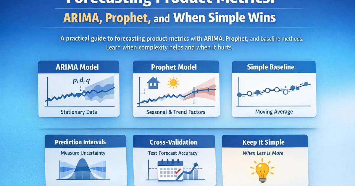
Forecasting Product Metrics: ARIMA, Prophet, and When Simple Wins

TL;DR

Product teams need forecasts for capacity planning, goal setting, anomaly detection, and resource allocation. This guide covers the practical forecasting toolkit: simple baselines that are surprisingly hard to beat, ARIMA for stationary patterns, Prophet for complex seasonality, and how to evaluate which method actually works for your data. The core lesson: always start simple, validate rigorously, and report uncertainty.

Why Forecast Product Metrics?

Forecasting serves four main purposes in product analytics:

1. Anomaly detection: A forecast defines "expected." Deviations from expected are anomalies worth investigating. See our overview of time series analysis for product metrics.
2. Goal setting: Realistic targets come from projecting current trajectories with uncertainty bounds.
3. Capacity planning: Infrastructure, support staffing, and inventory decisions require estimates of future demand.
4. Impact estimation: Comparing actual post-launch metrics to forecasted counterfactuals estimates causal impact (see interrupted time series).

Start Simple: Baseline Methods

Seasonal Naive

The seasonal naive forecast predicts next week using this week's values: next Monday = this Monday, next Tuesday = this Tuesday, and so on.

# Seasonal naive: use last week's values
def seasonal_naive(data, period=7, horizon=7):
    return data[-period:(-period + horizon)]

This method captures weekly seasonality perfectly and requires zero parameters. It is your minimum bar -- any method that cannot beat seasonal naive is not worth the complexity.

Moving Average

Average the last $k$ periods to smooth out noise:

def moving_average(data, window=28):
    return data[-window:].mean()

Moving averages are simple, interpretable, and provide a steady baseline. They lag behind trends but handle noise well.

Exponential Smoothing (ETS)

ETS is a family of methods that weight recent observations more heavily than older ones. The Holt-Winters variant handles trend and seasonality.

from statsmodels.tsa.holtwinters import ExponentialSmoothing

model = ExponentialSmoothing(
    daily_dau,
    trend='add',
    seasonal='add',
    seasonal_periods=7
).fit()

forecast = model.forecast(steps=14)

ETS is often the best balance of simplicity and accuracy for product metrics. It adapts to level changes, captures trends, and models seasonality -- all with a handful of parameters.

ARIMA: The Classical Workhorse

Core Concept

ARIMA (AutoRegressive Integrated Moving Average) models the metric as a function of its own past values (AR), past forecast errors (MA), and differencing (I) to achieve stationarity.

ARIMA($p$, $d$, $q$):

• $p$: Number of autoregressive terms (how many past values to use)
• $d$: Degree of differencing (how many times to difference for stationarity)
• $q$: Number of moving average terms (how many past errors to use)

When to Use ARIMA

ARIMA works well when:

• The data is (or can be made) stationary through differencing
• Autocorrelation patterns are clear in the ACF/PACF
• You have enough data (50+ observations minimum, 100+ preferred)

Auto-ARIMA: Let the Algorithm Choose

Manual ARIMA order selection (examining ACF/PACF plots to choose $p$, $d$, $q$) is an art. Auto-ARIMA automates this using information criteria (AIC/BIC):

from pmdarima import auto_arima

model = auto_arima(
    daily_dau,
    seasonal=True,
    m=7,  # weekly seasonality
    stepwise=True,
    suppress_warnings=True,
    error_action="ignore"
)

print(model.summary())
forecast, conf_int = model.predict(
    n_periods=14,
    return_conf_int=True
)

Auto-ARIMA searches through combinations of ($p$, $d$, $q$) and seasonal ($P$, $D$, $Q$, $m$) parameters, selecting the model that minimizes AIC. This is the recommended approach for practitioners.

SARIMA: Adding Seasonality

SARIMA extends ARIMA with seasonal terms: ARIMA($p$, $d$, $q$)($P$, $D$, $Q$)$_m$, where $m$ is the seasonal period. For daily data with weekly seasonality, $m = 7$.

The seasonal components capture patterns that repeat every $m$ periods (e.g., the Monday effect, the weekend dip). Auto-ARIMA handles seasonal selection automatically when you specify $m$.

Prophet: Designed for Business Metrics

Why Prophet?

Facebook's Prophet was built specifically for business time series forecasting. It handles:

• Multiple seasonalities: Weekly, monthly, and annual simultaneously
• Holiday effects: Specify holiday dates and Prophet models their impact
• Changepoints: Automatic detection of trend changes
• Missing data: Handles gaps without imputation
• Outliers: Robust fitting reduces outlier influence

Implementation

from prophet import Prophet

# Prepare data in Prophet format
df = pd.DataFrame({
    'ds': dates,
    'y': daily_dau
})

model = Prophet(
    yearly_seasonality=True,
    weekly_seasonality=True,
    daily_seasonality=False,
    changepoint_prior_scale=0.05  # regularize changepoints
)

# Add holidays
model.add_country_holidays(country_name='US')

model.fit(df)

# Forecast 14 days
future = model.make_future_dataframe(periods=14)
forecast = model.predict(future)

Prophet's Strengths and Weaknesses

Strengths:

• Minimal tuning required for reasonable forecasts
• Handles multiple seasonalities natively
• Built-in holiday modeling
• Interpretable components (trend, weekly, yearly, holidays)
• Scales to many time series

Weaknesses:

• Can overfit with too many changepoints (reduce changepoint_prior_scale)
• Does not model autocorrelation in residuals (unlike ARIMA)
• Less flexible than ARIMA for short-term, high-frequency patterns
• Assumes additive or multiplicative seasonality (not a mix)

When to Choose Prophet Over ARIMA

• Multiple seasonal periods (weekly + annual): Prophet handles this natively; ARIMA requires nested seasonal terms
• Holiday effects: Prophet models them directly; ARIMA needs manual dummy variables
• Non-technical users: Prophet requires less statistical knowledge
• Many time series: Prophet's defaults work reasonably across different metrics

Model Evaluation: Time Series Cross-Validation

Why Standard Cross-Validation Fails

Random train/test splits violate temporal order -- you would train on future data and predict the past. Time series cross-validation uses expanding or rolling windows that always train on past data and evaluate on future data.

from sklearn.model_selection import TimeSeriesSplit

tscv = TimeSeriesSplit(n_splits=5)
for train_idx, test_idx in tscv.split(data):
    train, test = data[train_idx], data[test_idx]
    # Fit on train, evaluate on test

Key Metrics

MAE (Mean Absolute Error): Average absolute forecast error. Interpretable in the metric's units.

MAPE (Mean Absolute Percentage Error): MAE as a percentage of actual values. Useful for comparing across metrics with different scales, but undefined when actuals are zero.

RMSE (Root Mean Squared Error): Penalizes large errors more than MAE. Use when big misses are disproportionately costly.

Coverage: What percentage of actual values fall within the prediction interval? For 95% intervals, coverage should be near 95%. If it is 80%, your intervals are too narrow.

Comparing Models

results = {}
for name, model_fn in models.items():
    errors = []
    for train_idx, test_idx in tscv.split(data):
        train, test = data[train_idx], data[test_idx]
        forecast = model_fn(train, len(test))
        errors.append(np.mean(np.abs(test - forecast)))
    results[name] = np.mean(errors)

# Choose the model with lowest average MAE
best_model = min(results, key=results.get)

Always include the seasonal naive baseline. If your sophisticated model cannot beat it, either the data lacks predictable structure or your model is misconfigured.

Prediction Intervals: The Honest Part

Point forecasts are nearly always wrong. Prediction intervals convey the uncertainty that decision-makers need.

A 95% prediction interval should contain the actual future value 95% of the time. If your intervals are too narrow (low coverage), your model is overconfident. If too wide, the forecast is not useful.

For capacity planning: use the upper bound of the prediction interval. For goal setting: use the point forecast with the interval as context. For anomaly detection: flag observations outside the interval.

When Simple Wins

Simple methods win when:

• The time series is short (< 50 observations): Complex models overfit
• The metric is noisy with weak patterns: No model can predict randomness
• The forecast horizon is very short (1-2 periods): Recent values dominate
• You need interpretability: Explaining "we used last week's values" is easier than "our SARIMA(1,1,1)(0,1,1)7 model indicates..."
• Speed matters: Simple methods compute in milliseconds

Start simple. Add complexity only when cross-validation shows measurable improvement. Document your comparison so stakeholders trust the choice.