Contents
Double/Debiased Machine Learning: Causal Effects with Flexible Models
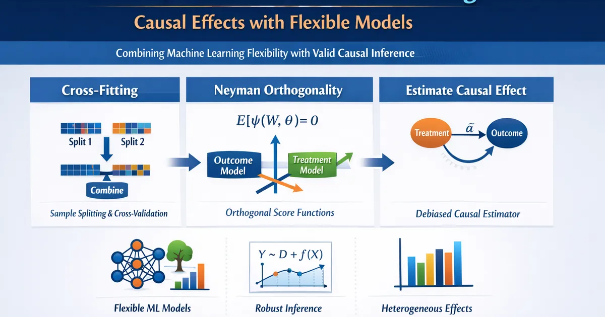
How double/debiased machine learning combines ML flexibility with valid causal inference. Learn cross-fitting, Neyman orthogonality, and practical DML workflows.
Quick Hits
- •Standard ML models optimize prediction, not causal estimation -- regularization bias and overfitting bias invalidate naive plug-in causal estimates
- •Double/debiased ML (DML) uses Neyman-orthogonal score functions and cross-fitting to produce root-n consistent causal estimates even with ML nuisance models
- •The 'double' refers to modeling both the outcome and the treatment as functions of confounders, then using residuals to estimate the causal effect
- •Cross-fitting (sample splitting) prevents overfitting bias without sacrificing sample size for the causal estimate
- •DML works with any ML method for the nuisance functions: random forests, gradient boosting, neural networks, or ensembles
TL;DR
Machine learning models are powerful predictors but terrible causal estimators out of the box. Regularization shrinks coefficients (biasing them), and overfitting on training data contaminates causal estimates. Double/debiased machine learning (DML) solves both problems by combining two insights: Neyman-orthogonal score functions that are insensitive to small errors in nuisance estimation, and cross-fitting that prevents overfitting bias. The result is a framework where you can use any ML model to handle complex confounding while still getting valid confidence intervals for causal effects. This post explains why naive ML fails for causal inference, how DML works, and how to implement it.
Why Machine Learning Fails at Causal Inference
The Regularization Bias Problem
ML models like LASSO, ridge regression, and gradient boosting use regularization to prevent overfitting. Regularization shrinks coefficients toward zero (or imposes other structural constraints). This is excellent for prediction -- it reduces variance at the cost of some bias.
But for causal inference, this bias is a problem. If you run a LASSO regression of outcomes on treatment and confounders, the treatment coefficient is regularized along with everything else. The resulting estimate is biased, and standard confidence intervals are invalid.
The Overfitting Bias Problem
Even without regularization, using the same data to estimate nuisance functions (the relationships between confounders and treatment/outcome) and the causal parameter creates overfitting bias. The nuisance model captures noise in the training data, and that noise leaks into the causal estimate.
This bias can be slow to vanish. With flexible ML models, overfitting bias can dominate the causal estimate even in large samples, making inference unreliable.
The Bottom Line
You cannot simply throw treatment into an ML model with confounders and interpret the output causally. The model is optimized for prediction, not for isolating causal variation.
How Double/Debiased ML Works
DML separates nuisance estimation from causal estimation using two key ideas.
Idea 1: Neyman Orthogonality
A score function for the causal parameter is Neyman orthogonal if small errors in nuisance estimation have only a second-order effect on the causal estimate. Formally, the pathwise derivative of the estimating equation with respect to the nuisance functions is zero at the true values.
This means: even if your ML models for the nuisance functions are somewhat wrong (as they always are), the causal estimate is barely affected.
Idea 2: Cross-Fitting
Cross-fitting is a form of sample splitting that prevents overfitting without wasting data.
- Split the data into folds (e.g., ).
- For each fold , estimate nuisance functions using all data except fold .
- Predict nuisance values for fold using the model trained on the other folds.
- Compute the causal estimate using the orthogonal score on the full sample with out-of-fold predictions.
Because predictions are always made on held-out data, overfitting bias is eliminated. Because all data contributes to the final estimate, there is no efficiency loss from sample splitting.
The Partially Linear Model: DML in Action
The simplest DML setup is the partially linear model:
Where:
- is the causal effect of treatment on outcome (the parameter of interest).
- is an arbitrary function of confounders (nuisance).
- is the conditional expectation of treatment given confounders (nuisance).
- are error terms.
The DML Algorithm
- Estimate : Use any ML model to predict from (ignoring ). Use cross-fitting.
- Estimate : Use any ML model to predict from . Use cross-fitting.
- Compute residuals:
- : the part of not explained by confounders.
- : the part of not explained by confounders.
- Regress on : The coefficient is the DML estimate of .
The intuition is Frisch-Waugh-Lovell on steroids: partial out the effect of confounders from both treatment and outcome using flexible ML, then estimate the causal effect from the cleaned residuals.
Why this works: By removing the confounders' influence from both and , the residual variation in is "as good as random" (conditional on the model being correct), and the coefficient on isolates the causal effect.
A Product Analytics Example
Context: You want to estimate the effect of using your company's mobile app (treatment) on monthly spending (outcome). You have 50 pre-treatment covariates including demographics, device info, browsing history, prior purchases, email engagement, and more. The relationships are likely nonlinear and interactive.
Approach:
- Outcome model: Train a gradient boosted tree to predict monthly spending from the 50 covariates (excluding app usage). Use 5-fold cross-fitting.
- Treatment model: Train a gradient boosted tree to predict app usage from the same covariates. Use 5-fold cross-fitting.
- Residualize: Compute (spending not explained by covariates) and (app usage not explained by covariates).
- Estimate: Regress on . The coefficient is your DML estimate of the causal effect of app usage on spending.
- Inference: Standard errors from the orthogonal score function provide valid confidence intervals.
Why DML here? With 50 covariates and complex relationships, a linear regression almost certainly misspecifies and . Propensity score matching struggles in high-dimensional covariate spaces. DML handles both problems gracefully.
Beyond Average Effects: Heterogeneous Treatment Effects
DML extends naturally to heterogeneous treatment effects -- estimating how the causal effect varies across subgroups or covariate values.
Conditional Average Treatment Effects (CATE)
Instead of estimating a single , estimate -- the treatment effect conditional on covariates . Methods include:
- Causal forests: Build a random forest that estimates using a modified splitting criterion (Wager and Athey, 2018).
- R-learner / DR-learner: Use DML-style residualization to construct a pseudo-outcome, then regress it on covariates to estimate heterogeneity.
- Generic ML (GML): Use any ML method on the pseudo-outcome.
Product application: Your mobile app's effect on spending may vary by user segment. DML-based CATE estimation can identify which segments benefit most, guiding targeted rollout decisions.
Practical Implementation
Software
- Python:
doubleml(official DML package),econml(Microsoft's causal ML library). - R:
DoubleML,grf(for causal forests).
Choosing ML Models for Nuisance Functions
Any model works in principle, but prefer:
- Gradient boosted trees (XGBoost, LightGBM): Strong default for tabular data with moderate dimensionality.
- Random forests: Robust and less prone to extreme predictions.
- Ensemble methods (stacking): Combine multiple learners for better nuisance estimation.
- LASSO/Elastic Net: Appropriate when the true nuisance functions are approximately sparse.
The nuisance models do not need to be perfect. They need to converge fast enough (typically at a rate or faster) for the orthogonality property to kick in.
Diagnostics
- Pre-treatment balance: After partialing out confounders, the residualized treatment should be uncorrelated with all covariates. Check this.
- Nuisance model performance: While prediction accuracy is not the end goal, extremely poor nuisance models suggest the confounders are not well captured. Monitor out-of-fold R-squared.
- Sensitivity analysis: DML still requires conditional ignorability (no unmeasured confounders). Use sensitivity analysis tools or argue substantively that the confounders are sufficient.
DML vs. Other Causal Methods
| Method | Functional form | Unmeasured confounders | High-dimensional covariates | Inference |
|---|---|---|---|---|
| OLS regression | Parametric (linear) | Requires conditional ignorability | Struggles | Standard |
| Propensity Score Matching | Semi-parametric | Requires conditional ignorability | Moderate | Bootstrap |
| Instrumental Variables | Semi-parametric | Handles (with instrument) | Moderate | Standard |
| DML | Flexible (any ML) | Requires conditional ignorability | Handles well | Orthogonal |
DML is the right tool when you need flexibility in modeling confounders and cannot rely on parametric assumptions. It does not solve the unmeasured confounding problem -- for that, you still need instrumental variables, regression discontinuity, or other structural approaches.
Limitations
Conditional ignorability is still required. DML relaxes functional form assumptions, not identification assumptions. If unmeasured confounders exist, DML is biased just like any other conditioning method.
Nuisance convergence rates matter. If your ML models converge too slowly (e.g., deep neural networks with limited data), the orthogonality property may not provide sufficient protection, and the causal estimate can be biased.
Complexity. DML is more complex to implement and explain than a simple regression. For stakeholders who need to understand the method, this can be a barrier.
Not a substitute for thinking. DML automates the functional form problem but not the causal reasoning problem. You still need a DAG, you still need to defend conditional ignorability, and you still need sensitivity analysis.
When to Reach for DML
Use DML when:
- You have rich, high-dimensional covariate data.
- The confounding relationships are likely nonlinear or interactive.
- You want valid confidence intervals (not just point predictions).
- Conditional ignorability is defensible.
For situations where identification does not rest on conditioning (thresholds, instruments, time variation), consider RDD, IV, or synthetic control instead. For the full landscape, see our causal inference overview.
References
- https://academic.oup.com/ectj/article/21/1/C1/5056401
- https://docs.doubleml.org/stable/
- https://arxiv.org/abs/1608.00060
Frequently Asked Questions
What is the advantage of DML over traditional regression?
What assumptions does DML require?
When should I use DML vs. propensity score matching?
Key Takeaway
Double/debiased machine learning brings the flexibility of modern ML to causal inference by separating nuisance estimation from causal parameter estimation, using orthogonal moments and cross-fitting to ensure valid inference even when nuisance models are complex.