Contents
Comparing Pre/Post Periods: Difference-in-Differences for Product
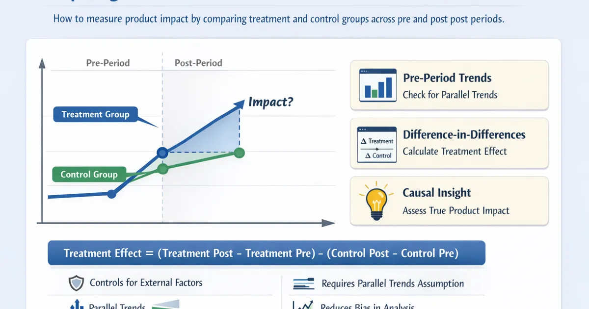
How to use difference-in-differences to measure product impact by comparing treatment and control groups across pre and post periods.
Quick Hits
- •DiD removes time-invariant confounders by differencing within groups AND across time
- •The key assumption is parallel trends -- treatment and control would have moved together without the intervention
- •DiD is stronger than simple pre/post comparison because it controls for external time trends
- •Always test the parallel trends assumption visually and statistically using pre-period data
- •Staggered rollouts complicate DiD -- use modern estimators designed for multi-period treatments
TL;DR
You rolled out a feature to one user segment but not another, and you want to measure the impact. Simple before-after comparison is confounded by time trends. Simple treatment-control comparison is confounded by group differences. Difference-in-differences (DiD) solves both by subtracting the control group's pre-post change from the treatment group's pre-post change. This guide covers the method, the critical parallel trends assumption, implementation, and common pitfalls in product analytics.
The Problem with Simple Comparisons
Pre/Post Is Biased
You launched a new recommendation algorithm on March 1 and engagement increased 8% from February to March. But engagement always increases in March because of seasonal patterns. How much of that 8% was the algorithm?
Treatment/Control Is Biased
Treatment users have 20% higher engagement than control users in March. But they also had 18% higher engagement in February. The groups are inherently different.
DiD Solves Both
DiD takes two differences:
First difference: Pre-post change within each group
- Treatment: March engagement - February engagement = +8%
- Control: March engagement - February engagement = +3%
Second difference: Difference in those changes
- DiD estimate = 8% - 3% = 5%
The 3% increase in the control group captures the external time trend (seasonality, other changes). By subtracting it, DiD isolates the treatment effect: 5%.
The DiD Setup
The 2x2 Table
| Pre-Period | Post-Period | Difference | |
|---|---|---|---|
| Treatment | |||
| Control | |||
| DiD = |
The Regression Framework
The standard DiD regression is:
Where:
- : Control group pre-period mean
- : Baseline difference between groups (pre-period)
- : Time effect (common to both groups)
- : The DiD treatment effect -- this is what you care about
import statsmodels.api as sm
import pandas as pd

# Prepare data with treatment, post, and interaction variables
df['treatment'] = (df['group'] == 'treatment').astype(int)
df['post'] = (df['date'] >= intervention_date).astype(int)
df['treatment_x_post'] = df['treatment'] * df['post']

# Fit DiD regression
X = sm.add_constant(df[['treatment', 'post', 'treatment_x_post']])
model = sm.OLS(df['engagement'], X).fit(
    cov_type='cluster',
    cov_kwds={'groups': df['user_id']}
)

print(f"DiD effect: {model.params['treatment_x_post']:.4f}")
print(f"p-value: {model.pvalues['treatment_x_post']:.4f}")
Clustered Standard Errors
When observations within a group are correlated (users observed over multiple days), standard errors should be clustered at the group level. This prevents artificially small standard errors and inflated significance.
The Parallel Trends Assumption
What It Means
DiD assumes that without the intervention, the treatment group would have followed the same trend as the control group. The two groups do not need the same level of the outcome -- they just need the same trajectory.
This is the most important assumption. If parallel trends fail, the DiD estimate is biased.
Testing Parallel Trends
Visual test: Plot the outcome for treatment and control groups over the pre-period. Do the lines move in parallel?
import matplotlib.pyplot as plt

pre_data = df[df['date'] < intervention_date]
for group in ['treatment', 'control']:
    group_data = pre_data[pre_data['group'] == group]
    daily_means = group_data.groupby('date')['engagement'].mean()
    plt.plot(daily_means.index, daily_means.values, label=group)

plt.axvline(x=intervention_date, color='red', linestyle='--')
plt.legend()
plt.title("Pre-Trend Check: Are Trends Parallel?")
plt.show()
Statistical test: Add group-specific time trends to the pre-period regression and test whether their coefficients differ:
pre_df = df[df['date'] < intervention_date].copy()
pre_df['time'] = (pre_df['date'] - pre_df['date'].min()).dt.days
pre_df['treatment_x_time'] = pre_df['treatment'] * pre_df['time']

X = sm.add_constant(pre_df[['treatment', 'time', 'treatment_x_time']])
model = sm.OLS(pre_df['engagement'], X).fit()

# If treatment_x_time is significant, parallel trends fails
print(f"Differential pre-trend: {model.params['treatment_x_time']:.4f}")
print(f"p-value: {model.pvalues['treatment_x_time']:.4f}")
A significant coefficient on treatment_x_time means the groups were already diverging before the intervention -- your DiD estimate will be biased.
Event Study Plot
The event study (or leads-and-lags) plot is the gold standard for assessing parallel trends. It estimates the DiD effect at each time point relative to the intervention:
# Create relative time dummies
df['rel_time'] = (df['date'] - intervention_date).dt.days
time_dummies = pd.get_dummies(df['rel_time'], prefix='t')
# Drop one pre-period as reference (e.g., t=-1)

interactions = time_dummies.multiply(df['treatment'], axis=0)
Pre-intervention coefficients should be near zero (no pre-trend difference). Post-intervention coefficients show the dynamic treatment effect.
Product Analytics Applications
Geographic Rollouts
You launch a feature in the US but not Europe. US users are the treatment group; European users are the control. DiD estimates the feature effect while controlling for global trends affecting both markets.
Caution: US and European users may have different seasonal patterns (parallel trends violation). Include day-of-week and holiday controls.
Segment-Based Rollouts
You enable a feature for paid users but not free users. DiD compares the pre-post change in engagement for paid vs. free users.
Caution: Paid and free users may respond differently to external events (e.g., a price change affects paid users more). Consider whether external shocks could differentially affect the groups.
Platform-Specific Launches
You ship a feature on iOS but not Android. DiD compares the change across platforms.
Caution: Platform-specific trends (OS updates, app store changes) can violate parallel trends. Always check pre-period trends carefully.
Advanced DiD: Staggered Adoption
The Problem
When treatment rolls out to different groups at different times (a staggered rollout), the standard 2x2 DiD breaks down. Groups treated earlier serve as controls for groups treated later, but they are already treated -- creating a contaminated control.
Recent econometrics research has shown that the standard two-way fixed effects (TWFE) regression can produce biased estimates with staggered treatment timing, especially when treatment effects vary across groups or over time.
Modern Solutions
Callaway and Sant'Anna (2021): Estimates group-time average treatment effects for each cohort (defined by treatment timing) and aggregates them.
Sun and Abraham (2021): Uses interaction-weighted estimators that avoid the contaminated control problem.
de Chaisemartin and D'Haultfoeuille (2020): Provides estimators robust to heterogeneous treatment effects.
For product teams doing staggered rollouts, the key takeaway is: do not use the standard TWFE regression. Use one of the modern estimators, or analyze each cohort separately and aggregate.
DiD vs. Other Methods
| Method | When to Use | Advantage |
|---|---|---|
| DiD | Treatment and control groups, pre/post data | Controls for time trends and group differences |
| ITS | No control group, one time series with intervention | Works without a control group |
| A/B test | Randomized treatment assignment | Gold standard for causal inference |
| Synthetic control | One treated unit, many potential controls | Constructs optimal weighted control |
DiD is stronger than ITS when a control group is available because it controls for common external shocks. It is weaker than a randomized A/B test because it relies on the parallel trends assumption rather than randomization.
Common Mistakes
Not checking parallel trends. This is the most common and most damaging mistake. If trends are not parallel pre-intervention, the DiD estimate is biased in an unknown direction. Always check.
Using too short a pre-period. A few days of parallel pre-trends do not guarantee the assumption holds. Use as much pre-period data as available and look for divergence at different time scales.
Ignoring anticipation effects. If treatment users change behavior before the official launch (because they heard about it, or because of pre-launch testing), the parallel trends assumption is violated in the pre-period. Look for pre-period divergence near the treatment date.
Forgetting to cluster standard errors. Observations within the same user or group are not independent. Failing to cluster inflates significance and produces false positives.
Applying standard DiD to staggered rollouts. As discussed above, TWFE with staggered treatment timing produces biased estimates. Use modern estimators designed for this case.
References
- https://doi.org/10.1257/jep.25.3.31
- https://diff.healthpolicydatascience.org/
- https://theeffectbook.net/ch-DifferenceinDifference.html
- Angrist, J. D., & Pischke, J. S. (2009). *Mostly Harmless Econometrics: An Empiricist's Companion*. Princeton University Press.
- Cunningham, S. (2021). *Causal Inference: The Mixtape*. Yale University Press.
Frequently Asked Questions
What's the difference between DiD and a simple pre/post comparison?
How do I find a good control group for DiD?
What if the parallel trends assumption is violated?
Key Takeaway
Difference-in-differences is the standard method for comparing treatment and control groups across pre and post periods. It controls for both group-level differences and time trends by taking two differences. The parallel trends assumption is critical -- always verify it with pre-period data before trusting DiD results.