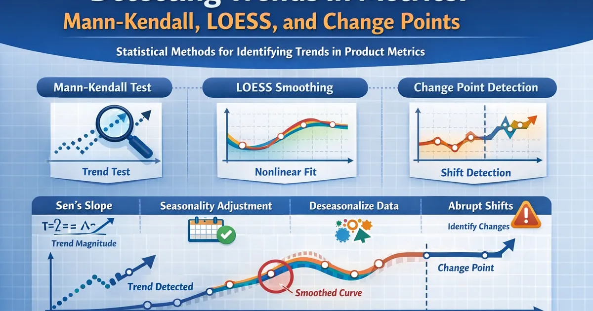
Detecting Trends in Metrics: Mann-Kendall, LOESS, and Change Points

TL;DR

A chart that "looks like it's going up" is not a trend -- it could be noise, seasonality, or a random walk. This guide covers three complementary methods for detecting genuine trends in product metrics: the Mann-Kendall test for statistical significance, LOESS smoothing for visualizing trend shape, and change point detection for finding abrupt shifts. Together, they give you a rigorous framework for answering the question every stakeholder asks: "Is this metric actually trending?"

The Problem: Eyeballing Is Not Trend Detection

Product teams look at dashboards and see lines going up or down. "DAU is trending up this month!" But is it really? With noisy daily data, short time horizons, and seasonal patterns, the human eye is remarkably bad at distinguishing genuine trends from randomness.

Consider: if you flip a coin 30 times and plot the cumulative sum, you will often see what looks like a clear trend -- even though the process is entirely random. Product metrics are noisier and more complex than coin flips.

You need statistical methods that answer: "Given the noise in this data, is there statistically significant evidence of a directional trend?"

Mann-Kendall Test: The Robust Trend Test

How It Works

The Mann-Kendall test is a non-parametric test for monotonic trends. It compares every pair of observations and counts whether later values tend to be larger or smaller than earlier values.

For each pair $(x_i, x_j)$ where $j > i$, it computes the sign of the difference. If more pairs show increases than decreases, there is evidence of an upward trend.

Key properties:

• No assumption of linearity or normality
• Robust to outliers (based on ranks, not magnitudes)
• Works with missing data
• Well-established significance testing

import pymannkendall as mk

# Test for trend in daily active users
result = mk.original_test(daily_dau)
print(f"Trend: {result.trend}")
print(f"p-value: {result.p}")
print(f"Kendall's tau: {result.Tau}")

Interpreting results:

• p-value < 0.05: Statistically significant trend
• Kendall's tau: Strength of trend (-1 to +1). Values near 0 mean no trend; near +1 or -1 mean strong monotonic trend
• Trend direction: "increasing", "decreasing", or "no trend"

Handling Seasonality: Seasonal Mann-Kendall

Standard Mann-Kendall can be fooled by seasonality. If your daily data has strong weekly cycles, the test might detect seasonality rather than trend.

The seasonal Mann-Kendall test solves this by applying the test separately within each season (e.g., comparing all Mondays to each other, all Tuesdays to each other) and combining results using a covariance correction.

# Seasonal Mann-Kendall with period=7 for weekly seasonality
result = mk.seasonal_test(daily_dau, period=7)

This is the version you should use for most product metrics with daily granularity.

Quantifying Trend Magnitude: Sen's Slope

Mann-Kendall tells you whether a trend exists. Sen's slope estimator tells you how fast the metric is changing. It computes the median slope across all pairs of observations, making it far more robust to outliers than ordinary least squares regression.

# Sen's slope is included in the pymannkendall output
print(f"Sen's slope: {result.slope} units per day")
print(f"Intercept: {result.intercept}")

If Sen's slope is 15.2 and your metric is DAU, the trend is roughly 15 additional users per day, or about 105 per week.

LOESS Smoothing: Seeing the Trend Shape

Beyond Linear Trends

Mann-Kendall detects monotonic trends, but many product metrics have nonlinear trends: growth that accelerates, plateaus, or reverses. LOESS (Locally Estimated Scatterplot Smoothing) fits local polynomial regressions across the time series, revealing the trend shape without assuming any functional form.

import statsmodels.api as sm

# LOESS smoothing
lowess = sm.nonparametric.lowess
smoothed = lowess(daily_dau, time_index, frac=0.15)

The frac parameter controls smoothness:

• Small frac (0.05-0.10): More responsive, captures short-term fluctuations
• Large frac (0.20-0.50): Smoother, emphasizes long-term direction
• Rule of thumb: Start with 0.15-0.20 and adjust visually

LOESS as a Decomposition Tool

LOESS is the "L" in STL decomposition. When you run STL, the trend component is estimated using LOESS. You can use LOESS directly for trend estimation, or indirectly through STL, which also separates out the seasonal component. See our guide on seasonal decomposition for the full STL approach.

Confidence Bands

LOESS smoothing alone does not provide uncertainty estimates. To add confidence bands, use bootstrapping: resample the residuals, re-fit LOESS, and collect the distribution of smoothed values at each time point. If the confidence band for the trend slope includes zero at any point, the trend is uncertain in that region.

Change Point Analysis: Finding Abrupt Shifts

When Trends Are Actually Level Shifts

Sometimes what appears to be a trend on a chart is actually a step change: the metric was flat, then jumped (or dropped) to a new level and stayed flat again. Traditional trend tests can detect this, but they do not pinpoint when the shift occurred.

Change point detection methods find the moment(s) where the statistical properties of the series (mean, variance, or both) changed. For a comprehensive treatment, see our guide on change point detection.

Key Methods

CUSUM (Cumulative Sum): Computes the cumulative deviation from the mean. A change point appears as a change in the slope of the CUSUM chart.

PELT (Pruned Exact Linear Time): Efficiently finds the optimal number and location of change points by minimizing a penalized cost function.

Bayesian Online Change Point Detection (BOCPD): Provides a probability of a change point at each time step, useful for real-time monitoring.

import ruptures as rpt

# PELT change point detection
algo = rpt.Pelt(model="rbf").fit(daily_dau.values)
change_points = algo.predict(pen=10)

Putting It All Together: A Practical Workflow

When a stakeholder asks "Is our DAU trending up?", follow this workflow:

1. Plot the raw data. Look for obvious patterns, outliers, and seasonality.
2. Deseasonalize using STL decomposition if seasonal patterns are present.
3. Run seasonal Mann-Kendall on the original data (or standard Mann-Kendall on deseasonalized data). Report the p-value and Kendall's tau.
4. Estimate magnitude with Sen's slope. Translate to business terms: "DAU is increasing by approximately 150 users per week."
5. Visualize with LOESS to show the trend shape. Is growth linear, accelerating, or flattening?
6. Check for change points to determine whether the "trend" is actually one or more abrupt shifts.
7. Report honestly. "There is a statistically significant upward trend ($\tau = 0.34$, $p < 0.001$) with an estimated increase of 150 DAU per week. LOESS smoothing suggests the growth rate is decelerating. A change point was detected around March 15, corresponding to the onboarding redesign launch."

This is vastly more informative -- and defensible -- than "the line is going up."

When Mann-Kendall Is Not Enough

Mann-Kendall has limitations:

• It detects monotonic trends only. If the metric goes up then down, Mann-Kendall may report no trend. Use LOESS or piecewise methods instead.
• It requires the trend to be consistent across the entire time period. If the trend reversed partway through, consider splitting the data at the change point and testing each segment separately.
• With strong autocorrelation, the variance correction in Mann-Kendall becomes important. Use implementations that apply the Hamed and Rao (1998) variance correction for autocorrelated data.
• Very short time series (under 10 observations) have low power. Collect more data before concluding there is no trend.

The combination of Mann-Kendall (statistical test), LOESS (visualization), and change point detection (structural breaks) covers the vast majority of trend analysis needs for product metrics. Start with the formal test, explore with smoothing, and validate with change point analysis.

References

- https://www.statisticshowto.com/mann-kendall-trend-test/
- https://www.itl.nist.gov/div898/software/dataplot/refman2/auxillar/mankenda.htm
- https://doi.org/10.1016/j.jhydrol.2004.07.006
- Mann, H. B. (1945). Nonparametric tests against trend. *Econometrica*, 13(3), 245-259.
- Cleveland, W. S. (1979). Robust locally weighted regression and smoothing scatterplots. *Journal of the American Statistical Association*, 74(368), 829-836.
Frequently Asked Questions
Can I just use linear regression to detect a trend?
How do I handle seasonality when testing for trend?
What's the difference between a trend and a change point?
Key Takeaway
Trend detection requires statistical rigor beyond eyeballing a chart. Mann-Kendall provides a robust test for monotonic trends, LOESS reveals trend shape without parametric assumptions, and Sen's slope quantifies trend magnitude. Always account for seasonality and autocorrelation, and distinguish gradual trends from abrupt shifts.