Contents
Confounding: The One Thing That Breaks Every Observational Study
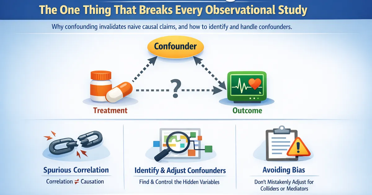
What confounding is, why it invalidates naive causal claims, and how to identify and handle confounders in product analytics and observational studies.
Quick Hits
- •A confounder is a variable that causally influences both the treatment and the outcome, creating a spurious association that is not the treatment effect
- •Confounding is the reason correlation does not imply causation -- it's the most common source of invalid causal claims in product analytics
- •Randomization eliminates confounding by design; observational methods must identify and adjust for confounders explicitly
- •Adjusting for the wrong variables (colliders, mediators) can introduce bias rather than remove it -- understanding causal structure is essential
- •You can never prove the absence of unmeasured confounders; sensitivity analysis quantifies how much hidden confounding would be needed to change your conclusion
TL;DR
Confounding is the reason that "users who do X have better outcomes" does not mean "X causes better outcomes." A confounder is a variable that affects both the treatment and the outcome, creating a non-causal association that masquerades as a treatment effect. Understanding confounding is the single most important skill for anyone doing causal inference with observational data. This post explains what confounders are, how they differ from colliders and mediators, how to identify them with DAGs, and what to do about them.
What Is Confounding?
Confounding occurs when a variable causes both the treatment and the outcome , creating an association between and that is not due to causing .
Example: Users who enable two-factor authentication (2FA) have 40% lower churn. Does enabling 2FA cause lower churn? Almost certainly not entirely. Users who enable 2FA are more security-conscious, more engaged, and more invested in the product. These characteristics independently predict lower churn. "Engagement" is a confounder: it drives both 2FA adoption and retention.
The causal DAG looks like this:
Engagement --> 2FA adoption
Engagement --> Retention
2FA adoption --> Retention (maybe a small true effect)
The observed 40% difference conflates the true causal effect of 2FA (which might be small) with the effect of engagement differences between the groups. This is confounding.
Why Randomization Solves Confounding
In a randomized experiment, you assign treatment randomly. This severs the causal arrow from every confounder to treatment. Engagement no longer predicts 2FA status because assignment is random. The only systematic difference between groups is the treatment itself.
This is why experiments are the gold standard. Not because they are statistically more powerful (they often are not), but because they structurally eliminate confounding -- including confounders you did not think of or cannot measure.
When you cannot randomize, you must deal with confounding explicitly. Every method in the causal inference toolkit is, at its core, a strategy for handling confounding.
Types of Variables: Confounders, Mediators, and Colliders
Not all variables between treatment and outcome behave the same way. Getting the type wrong does not just waste effort -- it introduces bias.
Confounders (Adjust for These)
A confounder causes both and . It creates a non-causal (backdoor) path between them. Adjusting for a confounder blocks this path and reduces bias.
C --> T
C --> Y
Action: Include confounders in your adjustment set (regression, matching, stratification).
Mediators (Do Not Adjust Unless Studying Mechanisms)
A mediator lies on the causal path from to . It is how the treatment produces its effect.
T --> M --> Y
Action: Do not adjust for mediators if you want the total effect. Adjusting for blocks the causal pathway and gives you only the direct effect. If you want to study mechanisms, see mediation analysis.
Colliders (Never Adjust Unless You Know What You Are Doing)
A collider is caused by both and (or by variables on separate paths from and ).
T --> D
Y --> D
Action: Do not adjust for colliders. Conditioning on a collider opens a spurious path between and (collider bias). This is one of the most counterintuitive results in causal inference: adding a control variable can create bias where none existed.
Example: Suppose both product quality () and marketing effectiveness () independently cause revenue (). Among high-revenue products (conditioning on ), quality and marketing become negatively associated -- if revenue is high and quality is low, marketing must be high. This spurious negative correlation is collider bias.
Identifying Confounders with DAGs
A directed acyclic graph (DAG) is a diagram of your causal assumptions. Each node is a variable, and each directed edge represents a causal relationship.
The Backdoor Criterion
Pearl's backdoor criterion provides a formal rule: a set of variables is sufficient to adjust for confounding if it blocks all backdoor paths from to without opening new ones (by conditioning on colliders).
Steps:
- Draw the DAG based on domain knowledge.
- Identify all paths from to .
- Separate causal paths (front-door, directed from to ) from non-causal paths (backdoor, with an arrow into ).
- Find a set that blocks every backdoor path.
- Verify that does not include any colliders on blocked paths, and does not include mediators (unless desired).
If you can find such a set and measure all variables in it, you can estimate the causal effect by adjusting for .
Common Confounding Patterns in Product Analytics
Self-Selection
Users choose to adopt features. The characteristics that drive adoption (engagement, sophistication, motivation) also drive the outcomes you measure (retention, revenue, satisfaction). This is the most pervasive confounder in product analytics.
Example: Users who complete an advanced tutorial have higher NPS. But completing the tutorial requires motivation and familiarity, which also predict NPS independent of the tutorial content.
Survivorship Bias
Analyzing only users who survived to a certain point (did not churn, completed onboarding) conditions on a post-treatment variable. Users who survived despite a bad experience may differ from those who survived with a good experience, creating confounded comparisons.
Time-Varying Confounding
Confounders may change over time and affect both treatment and outcomes at each time point. For example, a user's engagement at week 3 affects whether they use a feature at week 4 and also affects their retention. Standard adjustment methods may not handle this correctly; marginal structural models or G-estimation may be needed.
Ecological Confounding
Comparing aggregate units (markets, cohorts) can introduce confounders that do not exist at the individual level. A market with higher feature adoption and higher revenue may have a third factor (market maturity, internet penetration) driving both.
Simpson's Paradox: Confounding in Action
Simpson's paradox occurs when a trend present in subgroups reverses when the groups are combined. It is a direct manifestation of confounding.
Example: Overall, users who received the new dashboard have lower engagement. But within each segment (new users, mid-tenure users, veteran users), the new dashboard increases engagement. How?
The new dashboard was rolled out to a segment that has lower baseline engagement (new users are disproportionately in the treatment group). The apparent negative effect is confounded by user tenure. Within each tenure group, the effect is positive.
The solution: adjust for the confounder (user tenure). The lesson: always ask what variables might create misleading aggregate comparisons.
Dealing with Confounding
When You Can Measure Confounders
- Regression adjustment: Include confounders as covariates in a regression model.
- Propensity score matching: Match treated and untreated units on their propensity to receive treatment. See our PSM guide.
- Stratification: Divide the data into strata based on confounder values and estimate effects within strata.
- Inverse probability weighting: Reweight observations to create a pseudo-population where treatment is independent of confounders.
When You Cannot Measure Confounders
- Instrumental variables: Find exogenous variation in treatment. See IV methods.
- Regression discontinuity: Exploit threshold-based assignment. See RDD.
- Difference-in-differences: Use time variation with a control group. See synthetic control and DiD.
- Sensitivity analysis: Quantify how strong unmeasured confounding would need to be to invalidate your result.
When Confounding Is Intractable
Sometimes you simply cannot credibly adjust for confounding, and no structural feature of the data gives you a quasi-experiment. In these cases, the honest answer is: "We cannot make a causal claim. Here is the association, and here are the reasons it may not be causal." This is not a failure; it is intellectual honesty.
The Unmeasured Confounding Problem
You can never prove the absence of unmeasured confounders. Even with rich data, there is always a possible variable you did not observe. This is the fundamental limitation of all observational causal inference.
What you can do:
- Reason substantively. Given your domain knowledge, what are the most important confounders? Have you measured them?
- Compute the E-value. The E-value tells you the minimum strength of association an unmeasured confounder would need with both treatment and outcome (conditional on measured covariates) to fully explain away the observed effect.
- Run Rosenbaum bounds. For matched designs, quantify how sensitive your result is to hidden bias.
- Negative controls. Test your method on outcomes that should not be affected by treatment. If your method detects an "effect" on a negative control outcome, unmeasured confounding is likely present.
Key Principles
- Correlation is not causation because of confounding. This is not a platitude; it is the central problem of observational research.
- Not all variables are confounders. Adjusting for the wrong variable (collider, mediator) makes things worse, not better.
- DAGs before data. Draw your causal assumptions before you fit any model. Let the DAG guide your adjustment strategy.
- Unmeasured confounding cannot be ruled out. Report sensitivity analysis and be transparent about limitations.
- When in doubt, experiment. If the stakes are high and confounding is plausible, invest in running a proper randomized test.
For the complete toolkit of methods that address confounding in different ways, see our causal inference overview.
References
- https://www.hsph.harvard.edu/miguel-hernan/causal-inference-book/
- https://academic.oup.com/ije/article/31/1/163/655748
- https://ftp.cs.ucla.edu/pub/stat_ser/r350.pdf
Frequently Asked Questions
How do I know if a variable is a confounder?
What is the difference between confounding and selection bias?
Can I just control for everything?
Key Takeaway
Confounding is the single most important concept in observational causal inference. If you do not correctly identify and adjust for confounders -- and avoid adjusting for colliders and mediators -- your causal estimate will be biased no matter how large your sample or sophisticated your model.