Contents
Change Point Detection: When Did the Metric Shift?
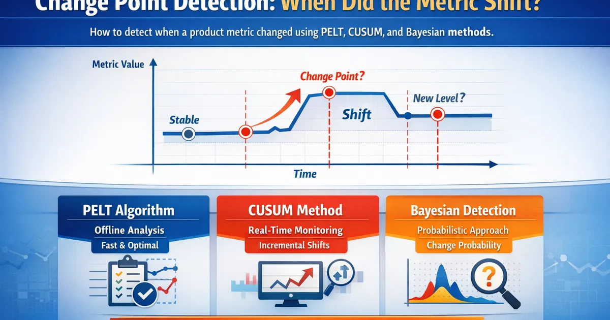
How to detect when a product metric changed using PELT, CUSUM, and Bayesian change point detection methods.
Quick Hits
- •Change point detection finds WHEN a metric's statistical properties shifted -- not just that they did
- •PELT is the go-to offline method: fast, optimal, and handles multiple change points
- •CUSUM charts are ideal for real-time monitoring of ongoing metric streams
- •Bayesian Online Change Point Detection gives probability of a change at each time step
- •Always validate detected change points against known events before reporting them as real
TL;DR
Product metrics shift. Sometimes you know why (a feature launched), sometimes you do not (something changed and you need to find when). Change point detection algorithms find the exact moments when a metric's statistical properties -- mean, variance, or distribution -- changed. This guide covers three main approaches: PELT for offline batch analysis, CUSUM for real-time monitoring, and Bayesian methods for probabilistic inference. Each has strengths suited to different product analytics scenarios.
What Is a Change Point?
A change point is a moment in time where the statistical properties of a time series change. Before the change point, the data follows one distribution; after it, a different one.
In product analytics, change points correspond to real events:
- A feature launch shifts average engagement upward
- A bug increases error rates overnight
- An algorithm update changes conversion rate distribution
- A competitor's action shifts user acquisition patterns
- A pricing change alters revenue per user
Change points differ from anomalies (single unusual points), trends (gradual movements), and seasonal effects (repeating patterns). A change point is an abrupt, persistent shift. See our pillar guide on time series analysis for how change points fit into the broader analytical framework.
PELT: The Offline Standard
How PELT Works
PELT (Pruned Exact Linear Time) finds the optimal set of change points by minimizing a cost function plus a penalty for each change point. It is exact (finds the globally optimal solution) and fast (linear time complexity through pruning).
The optimization problem is:
Where is the cost of fitting a segment, are the change point locations, is the number of change points, and is the penalty for adding a change point.
Implementation
import ruptures as rpt
import numpy as np

# Detect change points in daily conversion rate
signal = daily_conversion_rate.values

# PELT with RBF kernel cost function
algo = rpt.Pelt(model="rbf", min_size=7, jump=1)
algo.fit(signal)
change_points = algo.predict(pen=10)

print(f"Detected change points at indices: {change_points}")
Choosing the Cost Function
The cost function determines what kind of changes PELT detects:
model="l2": Detects changes in mean (Gaussian assumption). The most common choice for product metrics.model="rbf": Kernel-based. Detects changes in distribution without assuming a specific form. More flexible, slightly slower.model="normal": Detects changes in both mean and variance. Use when you suspect variance shifts (e.g., metric becomes more volatile).model="rank": Non-parametric, based on ranks. Robust to outliers but less powerful.
For most product metrics, start with "l2" (mean changes) or "rbf" (distribution changes).
Choosing the Penalty
The penalty controls sensitivity:
- Too low: Overfitting -- finds spurious change points in noise
- Too high: Underfitting -- misses real change points
- BIC penalty (): A principled default that balances fit and complexity
- Elbow method: Run PELT across a range of penalties and look for the "elbow" in the number of detected change points
# Using BIC penalty
n = len(signal)
pen_bic = np.log(n)
change_points = algo.predict(pen=pen_bic)
CUSUM: Real-Time Monitoring
How CUSUM Works
CUSUM (Cumulative Sum) charts accumulate deviations from a target value. When the cumulative sum exceeds a threshold, a change is detected.
For monitoring a product metric with known baseline mean :
Where is the allowance (half the shift size you want to detect) and triggers an alarm when it exceeds threshold .
Implementation
def cusum(data, target_mean, threshold=5, drift=0.5):
    """
    One-sided CUSUM for detecting upward shifts.
    """
    s_pos = [0]
    s_neg = [0]
    alarms = []

    for i, x in enumerate(data):
        s_pos.append(max(0, s_pos[-1] + (x - target_mean) - drift))
        s_neg.append(max(0, s_neg[-1] - (x - target_mean) - drift))

        if s_pos[-1] > threshold or s_neg[-1] > threshold:
            alarms.append(i)
            s_pos[-1] = 0  # reset after alarm
            s_neg[-1] = 0

    return alarms
When to Use CUSUM
CUSUM is ideal for:
- Ongoing monitoring dashboards where you need real-time alerts
- Quality control of metric streams (detecting degradation)
- Sequential detection where you process observations one at a time
- Known baselines where you want to detect departures from a specific value
CUSUM is less suited for retrospective analysis where you want to find all change points at once (use PELT instead).
Bayesian Online Change Point Detection (BOCPD)
How BOCPD Works
BOCPD computes the posterior probability of a change point at each time step. Instead of a binary "change or no change" answer, it gives you a probability: "there is a 73% probability that a change point occurred at time ."
The algorithm maintains a "run length" distribution -- the probability distribution over how long it has been since the last change point. When new data is inconsistent with the current run, the probability mass shifts to shorter run lengths, indicating a change.
Advantages
- Probabilistic output: Quantifies uncertainty about change point locations
- Online processing: Updates with each new observation
- No penalty tuning: The prior on run length replaces the penalty parameter
- Handles uncertainty: Multiple candidate change points can coexist with different probabilities
Implementation
import bayesian_changepoint_detection.online_changepoint_detection as oncd
from functools import partial

# Define hazard function (prior on segment length)
hazard = partial(oncd.constant_hazard, 250)  # mean segment length

# Run BOCPD
R, maxes = oncd.online_changepoint_detection(
    daily_dau.values,
    hazard,
    oncd.StudentT(0.1, 0.01, 1, 0)
)

# Extract most probable change points
change_prob = R[0, 1:]  # probability of change at each time
Practical Workflow: Finding What Changed and When
Step 1: Detect Change Points
Run PELT on the metric to identify candidate change points:
algo = rpt.Pelt(model="rbf", min_size=7).fit(signal)
change_points = algo.predict(pen=np.log(len(signal)))
Step 2: Cross-Reference with Events
For each detected change point, check:
- Was there a product release or feature launch?
- Did a marketing campaign start or end?
- Were there infrastructure changes?
- Did anything happen externally (holiday, competitor action, news event)?
Step 3: Quantify the Shift
For each confirmed change point, estimate the before/after difference:
# Simple before/after comparison at change point index cp
before = signal[max(0, cp-30):cp]
after = signal[cp:min(len(signal), cp+30)]
shift = np.mean(after) - np.mean(before)
print(f"Level shift: {shift:.2f}")
For formal statistical testing of the shift, see our guide on interrupted time series.
Step 4: Report
"Change point detection identified a shift in daily conversion rate on March 15 (from 4.2% to 4.7% average). This coincides with the checkout redesign launched on March 14. The estimated lift of 0.5 percentage points (12% relative) is consistent with the interrupted time series analysis."
Handling Seasonality
Change point algorithms can mistake seasonal transitions (weekday to weekend, summer to fall) as change points. To avoid this:
- Deseasonalize first: Apply STL decomposition and run change point detection on the trend + residual component.
- Use appropriate minimum segment size: Set
min_sizeto at least one full seasonal cycle (7 for daily data with weekly seasonality). - Validate against seasonal calendar: If detected change points consistently fall at seasonal boundaries, they are probably seasonal artifacts.
Multiple Change Points vs. Single Change Point
Some scenarios call for different approaches:
Single change point (you know one event happened): Use a likelihood ratio test or segmented regression. See interrupted time series.
Multiple change points (exploring what happened over a long period): Use PELT with automatic penalty selection. It finds the optimal number and locations simultaneously.
Ongoing monitoring (detecting the next change as it happens): Use CUSUM or BOCPD for sequential detection.
Common Pitfalls
Confusing change points with outliers. A single spike is not a change point. Verify that the shift persists for multiple time steps after the detected point.
Overfitting with too-low penalties. If PELT finds 15 change points in 90 days of data, your penalty is likely too low. Real product metrics rarely have that many genuine structural shifts.
Ignoring autocorrelation. Many change point methods assume independent observations. When applied to autocorrelated data, they may detect spurious change points. Deseasonalize and consider differencing before applying detection algorithms.
Not validating. Every detected change point should be cross-referenced with known events. An unexplained change point is a hypothesis to investigate, not a conclusion to report.
References
- https://centre-borelli.github.io/ruptures-docs/
- https://doi.org/10.1080/01621459.2012.737745
- https://doi.org/10.1111/j.1467-9868.2005.00532.x
- Killick, R., Fearnhead, P., & Eckley, I. A. (2012). Optimal detection of changepoints with a linear computational cost. *Journal of the American Statistical Association*, 107(500), 1590-1598.
- Adams, R. P., & MacKay, D. J. (2007). Bayesian online changepoint detection. *arXiv preprint arXiv:0710.3742*.
Frequently Asked Questions
How is change point detection different from anomaly detection?
Can change point detection find gradual changes?
How do I choose the sensitivity (penalty parameter)?
Key Takeaway
Change point detection pinpoints when a metric's behavior shifted, not just whether it did. PELT is efficient for offline batch analysis, CUSUM for real-time monitoring, and Bayesian methods for probabilistic assessments. Always cross-reference detected change points with known events and product changes to build a causal narrative.