Contents
Autocorrelation: Why Your Daily Metrics Aren't Independent
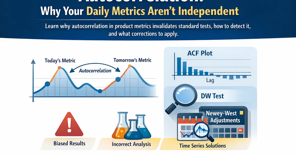
Learn why autocorrelation in product metrics invalidates standard tests, how to detect it, and what corrections to apply.
Quick Hits
- •If today's DAU is high, tomorrow's probably is too -- that's autocorrelation
- •Standard t-tests and confidence intervals assume independence and give wrong answers with autocorrelated data
- •The ACF plot is your go-to diagnostic -- check it before running any statistical test on time series
- •Newey-West standard errors correct for autocorrelation without changing your estimator
- •Weekly seasonality shows up as spikes at lags 7, 14, 21 in the ACF
TL;DR
Product metrics collected over time are almost never independent. Today's DAU is correlated with yesterday's, this week's revenue with last week's, and this month's churn with last month's. This autocorrelation violates the assumptions of standard statistical tests, leading to overconfident conclusions and inflated false positive rates. This guide explains what autocorrelation is, how to detect it, why it matters, and what to do about it.
What Is Autocorrelation?
Autocorrelation is the correlation of a variable with itself at different time lags. At lag 1, it measures how correlated today's value is with yesterday's. At lag 7, how correlated today is with the same day last week.
Formally, the autocorrelation at lag is:
For most product metrics, (lag-1 autocorrelation) is strongly positive, often 0.5 to 0.9. This means consecutive days share a substantial portion of their variance -- they are not independent observations.
Why Product Metrics Are Autocorrelated
The user base does not reset each day. The same people use your product today and tomorrow, creating inherent persistence. Specific causes include:
- User retention: Active users today are likely active tomorrow
- Subscription models: Revenue is sticky -- it changes slowly as subscribers join or leave
- Habit formation: Engagement patterns develop over weeks
- External persistence: Weather, economic conditions, and cultural events affect consecutive days similarly
- Platform algorithms: Recommendation systems create self-reinforcing feedback loops
Detecting Autocorrelation
The ACF Plot
The autocorrelation function (ACF) plot is the primary diagnostic tool. It displays the autocorrelation coefficient at each lag, along with significance bands (typically at ).
from statsmodels.graphics.tsaplots import plot_acf
import matplotlib.pyplot as plt

fig, ax = plt.subplots(figsize=(10, 4))
plot_acf(daily_dau, lags=30, ax=ax)
plt.title("ACF of Daily Active Users")
plt.show()
Reading the ACF plot:
- Lag 0 is always 1.0 (a variable perfectly correlates with itself)
- Slowly decaying values suggest a trend or strong persistence
- Spikes at regular intervals (7, 14, 21) indicate weekly seasonality
- Values exceeding the blue bands are statistically significant
- Alternating positive/negative values suggest oscillatory behavior
The Ljung-Box Test
The Ljung-Box test formally tests whether any of a group of autocorrelations are significantly different from zero. It is a portmanteau test -- it checks multiple lags simultaneously.
from statsmodels.stats.diagnostic import acorr_ljungbox

# Test first 10 lags
result = acorr_ljungbox(daily_dau, lags=10, return_df=True)
print(result)
A significant result (p < 0.05) means the data is autocorrelated. For product metrics, this is almost always significant -- the question is usually not whether autocorrelation exists, but how strong it is and what structure it has.
The Durbin-Watson Test
The Durbin-Watson statistic specifically tests for lag-1 autocorrelation in regression residuals. It ranges from 0 to 4:
- DW near 2: No autocorrelation
- DW near 0: Strong positive autocorrelation
- DW near 4: Strong negative autocorrelation (rare in practice)
from statsmodels.stats.stattools import durbin_watson

# After fitting a regression model
dw = durbin_watson(model.resid)
print(f"Durbin-Watson: {dw:.2f}")
Why It Matters: The Consequences of Ignoring Autocorrelation
Inflated False Positives
When you run a two-sample t-test comparing 30 days of metric values between two periods, the test treats each day as an independent observation, giving you 30 degrees of freedom. But if the lag-1 autocorrelation is 0.7, your effective sample size is far smaller -- perhaps 8-10 equivalent independent observations. The t-test's standard error is too small, the t-statistic is too large, and the p-value is too low.
The effective sample size under AR(1) autocorrelation is approximately:
With days and , that is roughly effective observations. Your test behaves as if you had 5 data points, not 30.
Misleading Confidence Intervals
Confidence intervals computed under the independence assumption are too narrow. When your dashboard shows "DAU: 50,000 +/- 200," those error bars may actually be +/- 800 once you account for autocorrelation. Decisions based on the narrow intervals are overconfident.
A/B Test Contamination
If you analyze A/B test results using daily metric values as independent data points, autocorrelation inflates your test statistics. A test that should have a 5% false positive rate may actually have 15-30% false positive rates. This is one reason why user-level randomization and analysis are preferred over time-based comparisons.
What to Do About It
Option 1: Aggregate Away the Problem
The simplest approach: aggregate your data to eliminate autocorrelation. Instead of analyzing 30 daily values, compute a single metric for the entire period. One mean per group has no autocorrelation issue.
This works well for A/B tests where you can compute one conversion rate per variant across the entire experiment. It loses temporal information but avoids autocorrelation entirely.
Option 2: Newey-West Standard Errors
Newey-West standard errors adjust for autocorrelation (and heteroskedasticity) without changing the point estimate. They increase the standard errors to reflect the reduced effective sample size.
import statsmodels.api as sm

# OLS with Newey-West corrected standard errors
model = sm.OLS(y, X).fit(cov_type='HAC',
                          cov_kwds={'maxlags': 7})
print(model.summary())
The maxlags parameter controls how many lags of autocorrelation to account for. For daily data with weekly seasonality, use at least 7.
Option 3: Autoregressive Models
Model the autocorrelation explicitly using autoregressive (AR) or ARIMA models. These models include lagged values as predictors, capturing the temporal dependence structure.
from statsmodels.tsa.arima.model import ARIMA

# AR(1) model
model = ARIMA(daily_dau, order=(1, 0, 0)).fit()
print(model.summary())
The residuals from a well-specified ARIMA model should be approximately uncorrelated. If they are, the autocorrelation has been properly accounted for.
Option 4: Differencing
First differencing (computing day-over-day changes instead of raw values) removes much of the autocorrelation. Instead of analyzing DAU levels, analyze daily DAU changes.
dau_diff = daily_dau.diff().dropna()
Differenced data often has much weaker autocorrelation than the raw series. However, differencing changes your question from "what is the level?" to "what is the rate of change?" -- make sure this is what you want to answer.
Partial Autocorrelation (PACF): Digging Deeper
While the ACF shows total correlation at each lag (including indirect correlations through intermediate lags), the partial autocorrelation function (PACF) isolates the direct correlation at each lag, removing the influence of intermediate lags.
The PACF is essential for model selection:
- ACF decays slowly, PACF cuts off after lag : Suggests an AR() model
- ACF cuts off after lag , PACF decays slowly: Suggests an MA() model
- Both decay gradually: Suggests an ARMA or ARIMA model
from statsmodels.graphics.tsaplots import plot_pacf

fig, ax = plt.subplots(figsize=(10, 4))
plot_pacf(daily_dau, lags=30, ax=ax, method='ywm')
plt.title("PACF of Daily Active Users")
plt.show()
Understanding the PACF helps you build forecasting models, which is covered in our guide on forecasting product metrics.
Practical Checklist
Before running any statistical test on time series product data:
- Plot the ACF for at least 30 lags. Is it significant beyond lag 0?
- Run the Ljung-Box test as a formal check.
- If autocorrelation is present (it almost certainly is):
- For simple comparisons: aggregate to one number per group
- For regression: use Newey-West standard errors
- For modeling: fit an ARIMA or similar time series model
- For A/B tests: prefer user-level analysis over daily aggregates
- Verify your correction worked by checking ACF of residuals.
- Report the autocorrelation so readers understand why you used corrected methods.
Autocorrelation is not a problem to fear -- it is a property to respect. Acknowledging it leads to more honest and accurate analyses. Ignoring it leads to the kind of overconfident claims that erode trust in your data team.
References
- https://otexts.com/fpp3/acf.html
- https://www.statsmodels.org/stable/generated/statsmodels.stats.diagnostic.acorr_ljungbox.html
- https://en.wikipedia.org/wiki/Newey%E2%80%93West_estimator
- Newey, W. K., & West, K. D. (1987). A simple, positive semi-definite, heteroskedasticity and autocorrelation consistent covariance matrix. *Econometrica*, 55(3), 703-708.
- Box, G. E. P., & Jenkins, G. M. (1976). *Time Series Analysis: Forecasting and Control*. Holden-Day.
Frequently Asked Questions
What causes autocorrelation in product metrics?
Can I just ignore autocorrelation?
How does autocorrelation affect A/B test analysis?
Key Takeaway
Autocorrelation is nearly universal in product metrics and violates the independence assumption of most standard statistical tests. Always check the ACF plot before running tests on time series data, and use corrections like Newey-West standard errors or time-series-aware methods when autocorrelation is present.