Contents
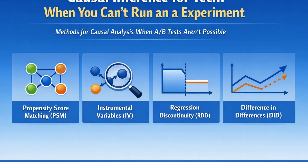
Causal Inference for Tech: When You Can't Run an Experiment
A practical guide to causal inference methods for product and data analysts when A/B tests aren't possible. Covers PSM, IV, RDD, DiD, and more.
Quick Hits
- •A/B tests are the gold standard, but ethical, legal, or practical constraints make them impossible for roughly 30-50% of the questions product teams need answered
- •Every observational causal method is fighting the same enemy: selection bias from non-random treatment assignment
- •Propensity score matching, instrumental variables, regression discontinuity, and difference-in-differences each exploit a different structural assumption to recover causal estimates
- •No method is assumption-free; the right choice depends on the data-generating process, not your personal comfort level
- •Sensitivity analysis is non-negotiable: always ask how strong unmeasured confounding would need to be to overturn your conclusion
TL;DR
A/B tests are the cleanest way to measure cause and effect, but you can't always run one. Causal inference methods let you draw credible causal conclusions from observational data by exploiting structural features of how treatment was assigned. This guide covers why experiments fail, the core challenge of selection bias, and the five most important methods for product and data analysts: propensity score matching, instrumental variables, regression discontinuity, difference-in-differences, and synthetic control. Each method requires different assumptions; choosing well means understanding your data-generating process, not running the trendiest technique.
Why Experiments Aren't Always Possible
Randomized experiments are the gold standard for causal inference because they eliminate confounding by design. When you randomly assign users to treatment and control, every other variable -- observed and unobserved -- is balanced on average between groups. Any difference in outcomes can be attributed to the treatment.
But product teams regularly face situations where experiments are off the table:
Ethical constraints. You cannot randomly deny users a safety feature or a legally mandated disclosure. If your feature prevents fraud, withholding it from a control group creates real harm.
Already-launched changes. The feature shipped to everyone six months ago. Leadership now wants to know if it worked. There is no control group and no time machine.
Infrastructure limitations. Some changes -- like a new pricing model or a server migration -- affect everyone simultaneously. There is no way to randomize at the user level.
Business pressure. Sometimes the organization simply will not wait for an experiment to reach statistical power. A product leader wants an answer by Friday, and the feature has already been rolled out to certain markets.
Network effects. When users interact with each other, randomizing at the individual level creates spillover. A user in the control group may be affected by treated users in their network, violating the Stable Unit Treatment Value Assumption (SUTVA).
In all these cases, you need methods that extract causal estimates from non-experimental data. That is the domain of causal inference.
The Core Challenge: Selection Bias and Confounding
The fundamental problem with observational data is that treatment assignment is not random. Users who adopt a feature differ systematically from users who do not. Power users opt in first. Engaged customers respond to nudges. High-value accounts get personal onboarding.
This means any naive comparison of outcomes between treated and untreated groups conflates the treatment effect with pre-existing differences. If users who activated the premium tier have higher retention, is that because the tier is effective, or because users who were already committed are more likely to upgrade?
This is confounding: a variable that influences both treatment assignment and the outcome, creating a spurious association. The entire field of observational causal inference exists to handle confounding.
There are two broad strategies:
-
Condition on confounders. If you can measure everything that jointly affects treatment and outcome, you can adjust for it. Propensity score matching and regression adjustment take this approach. The critical assumption is "no unmeasured confounders" (conditional ignorability).
-
Exploit structural features. If the data has a natural experiment embedded in it -- a threshold, an external shock, a time-based rollout -- you can use that structure to recover a causal estimate even with unmeasured confounders. Instrumental variables, regression discontinuity, and difference-in-differences take this approach.
Neither strategy is assumption-free. The question is always: which assumptions are most defensible given your specific context?
The Five Key Methods
Propensity Score Matching (PSM)
When to use it: You have rich user-level covariates and believe you can measure all relevant confounders.
Propensity score matching estimates the probability of receiving treatment given observed covariates, then matches treated users to similar untreated users based on that score. By comparing outcomes within matched pairs, you approximate what a randomized experiment would have shown.
Example: You rolled out a coaching feature to users who opted in. You have demographics, tenure, engagement history, and plan type. You match each opted-in user to an opted-out user with a similar propensity score and compare retention rates.
Key assumption: No unmeasured confounders. If motivation or technical savviness drives both opt-in and retention, and you cannot measure them, your estimate is biased. Read more in our deep dive on propensity score matching.
Instrumental Variables (IV)
When to use it: You have an exogenous variable that affects whether users receive treatment but does not directly affect the outcome.
Instrumental variables work by finding a source of variation in treatment that is "as good as random." The instrument predicts treatment status but only affects the outcome through the treatment itself.
Example: You want to know if using your mobile app increases purchases. You use a push notification A/B test as an instrument: the notification randomly encourages app usage, but the notification itself does not directly cause purchases. The notification affects purchases only through increased app usage. See our guide on instrumental variables in product data.
Key assumption: The exclusion restriction -- the instrument affects the outcome only through treatment. This is untestable and must be argued substantively.
Regression Discontinuity Design (RDD)
When to use it: Treatment is assigned based on whether a continuous variable crosses a threshold.
RDD exploits the fact that observations just above and just below a cutoff are nearly identical on all characteristics except treatment status. Comparing outcomes near the cutoff gives a local causal estimate.
Example: Users with an engagement score above 80 get a loyalty reward. Comparing users scoring 79 to those scoring 81 isolates the reward's effect, since these users are otherwise almost indistinguishable. Explore this further in our post on regression discontinuity design.
Key assumption: Users cannot precisely manipulate their score to cross the threshold. If they can game the system, the comparison breaks down.
Difference-in-Differences (DiD)
When to use it: You have before-and-after data for a treatment group and a comparison group that did not receive treatment.
DiD compares the change in outcomes over time between the treated group and the untreated group. It removes time-invariant confounders and common time trends, isolating the treatment effect.
Example: You launched a redesigned checkout flow in the US but not in Canada. By comparing the change in conversion rates in the US (before vs. after) to the change in Canada (same period), you estimate the redesign's causal impact.
Key assumption: Parallel trends -- absent treatment, both groups would have followed the same trajectory. This is testable in pre-treatment periods but fundamentally unverifiable in the post-treatment window.
Synthetic Control
When to use it: You have a single treated unit (often a region or market) and a pool of untreated units.
Synthetic control builds a weighted combination of untreated units that closely matches the treated unit's pre-treatment trajectory. The post-treatment divergence between the treated unit and its synthetic counterpart estimates the causal effect.
Example: You launched a new pricing model in Germany. Using pre-launch revenue trends from France, Spain, Italy, and the Netherlands, you construct a "synthetic Germany" that tracks the real Germany's revenue before launch. Post-launch divergence measures the pricing model's effect. Learn more in our post on synthetic control for geo tests.
Key assumption: The donor pool can reproduce the treated unit's pre-treatment behavior, and no other intervention occurred simultaneously.
Choosing the Right Method
The right method depends on the structure of your data, not your preference:
| Scenario | Best method |
|---|---|
| Rich covariates, conditional ignorability defensible | Propensity Score Matching |
| Exogenous instrument available | Instrumental Variables |
| Treatment assigned by a threshold | Regression Discontinuity |
| Before/after data with untreated comparison group | Difference-in-Differences |
| Single treated unit, many donors | Synthetic Control |
Often, the best approach is to use multiple methods and check whether they converge on a similar estimate. Agreement across methods with different assumptions is strong evidence that the causal effect is real.
The Role of DAGs and Assumptions
Every causal method encodes assumptions about how variables relate to each other. Directed acyclic graphs (DAGs) make those assumptions explicit. Before fitting any model, draw the causal structure: which variables cause which, where confounders enter, and what paths need to be blocked.
A DAG will tell you which variables to condition on (and which to leave alone). Conditioning on a collider -- a variable caused by both treatment and outcome -- opens a spurious path and introduces bias. Conditioning on a mediator blocks the very causal pathway you are trying to estimate. Getting the DAG wrong means getting the analysis wrong, regardless of how sophisticated your estimator is.
Understanding confounding is the single most important skill for observational causal inference.
Sensitivity Analysis: How Robust Is Your Estimate?
No observational study can completely rule out unmeasured confounding. Sensitivity analysis asks: how strong would an unmeasured confounder need to be to change my conclusion?
Methods like Rosenbaum bounds (for matched designs) and the E-value (for general settings) quantify this. If your result would be overturned by a confounder with a risk ratio of 1.2, you should be worried. If it would take a confounder with a risk ratio of 5, you can be more confident.
Always report sensitivity analysis alongside your point estimate. It transforms the conversation from "Is the estimate unbiased?" (unknowable) to "How much bias would be needed to invalidate it?" (quantifiable).
Practical Workflow for Product Analysts
- Define the causal question precisely. What is the treatment? What is the outcome? What is the population?
- Draw a DAG. Make your assumptions explicit before touching data.
- Assess data structure. What does the assignment mechanism look like? Is there a threshold, instrument, or natural comparison group?
- Choose the method that matches your structure. Do not force a method onto data that does not support it.
- Check assumptions. Balance tests, placebo checks, parallel trend diagnostics, falsification tests.
- Run sensitivity analysis. Report how robust your estimate is to violations of key assumptions.
- Communicate uncertainty. A range of plausible effects is more honest and more useful than a single point estimate.
Where to Go Next
This pillar post gives you the map. The supporting posts in this cluster give you the details:
- Propensity Score Matching: balancing groups without randomization
- Instrumental Variables: finding natural experiments in product data
- Regression Discontinuity: when thresholds create experiments
- Difference-in-Differences and Synthetic Control: building counterfactuals for geo tests
- Confounding: the variable that breaks everything
- DAGs for Analysts: drawing assumptions before analyzing
- Mediation Analysis: understanding causal mechanisms
- Double/Debiased ML: flexible causal estimation with machine learning
Causal inference is harder than experimentation. But when an experiment is not an option, these methods -- applied with care, skepticism, and transparency -- are the best tools available.
References
- https://www.hsph.harvard.edu/miguel-hernan/causal-inference-book/
- https://mixtape.scunning.com/
- https://matheusfacure.github.io/python-causality-handbook/
Frequently Asked Questions
When should I use causal inference instead of an A/B test?
Which causal inference method should I use?
How do I know if my causal estimate is valid?
Key Takeaway
Causal inference methods let you estimate cause-and-effect from observational data when experiments are impossible, but each method comes with assumptions that must be defended, not just assumed. The best analysts match the method to the data structure and rigorously test those assumptions.